三维点云处理(7)——Deep Learning

Introduction

Perceptron Optimization (Neural Network)

A Perceptron:$y=w^{T}x+b$, Modify weight $w$ such that $\hat{y}$ gets ‘closer’ to $y$.

• Deep learning is trying to solve one problem:
  $$\underset{x}{\min }f(x),y=f(x)=w^{T}x+b$$
• It is a linear regression problem
  $$w=\arg \underset{w}{\min }\sum _{i=1}^M\frac{1}{2}(w^T{x}_i-y_i{)}^2$$
  • Features $x_i\in {\mathbb{R}}^n$
  • Ground truth $y_i\in \mathbb{R}$
• Typical $Ax=b$ problem, but we can solve it by Gradient Descent
  $$x^{\ast }=\arg \underset{x}{\min }F(x),x_{n+1}=x_n-\gamma \nabla F(x_n)$$
  • $\gamma$ is the step size
  • $\nabla F(x_n)$ is the gradient of $F$ at $x_n$

Chain Rule

$$f(x)=g(u),u=h(x)\to f^{\prime }(x)=g^{\prime }(u)h^{\prime }(x)$$

Matrix Calculus

Denominator layout:
$$\frac{\partial \mathbf{y}}{\partial x}\in {\mathbb{R}}^{1\times m},\frac{\partial y}{\partial \mathbf{x}}={\mathbb{R}}^n$$
Numerator layout:
$$\frac{\partial \mathbf{y}}{\partial x}\in {\mathbb{R}}^m,\frac{\partial y}{\partial \mathbf{x}}={\mathbb{R}}^{1\times n}$$
$\mathbf{x}\in {\mathbb{R}}^n,\mathbf{y}\in {\mathbb{R}}^m,\mathbf{X}\in {\mathbb{R}}^{n\times m},\mathbf{Y}\in {\mathbb{R}}^{m\times n}$
$$\frac{\partial y}{\partial \mathbf{x}}=\left[\begin{array}{c}\frac{\partial y}{\partial x_1}\\ \frac{\partial y}{\partial x_2}\\ ⋮\\ \frac{\partial y}{\partial x_n}\end{array}\right],\frac{\partial \mathbf{y}}{\partial x}=\left[\begin{array}{cccc}\frac{\partial y_1}{\partial x}& \frac{\partial y_2}{\partial x}& \cdots & \frac{\partial y_n}{\partial x}\end{array}\right]$$
$$\frac{\partial \mathbf{y}}{\partial \mathbf{x}}=\left[\begin{array}{cccc}\frac{\partial y_1}{\partial x_1}& \frac{\partial y_2}{\partial x_1}& \cdots & \frac{\partial y_m}{\partial x_1}\\ \frac{\partial y_1}{\partial x_2}& \frac{\partial y_2}{\partial x_2}& \cdots & \frac{\partial y_m}{\partial x_2}\\ ⋮& ⋮& \ddots & ⋮\\ \frac{\partial y_1}{\partial x_n}& \frac{\partial y_2}{\partial x_n}& \cdots & \frac{\partial y_m}{\partial x_n}\end{array}\right]$$
$$\frac{\partial y}{\partial \mathbf{X}}=\left[\begin{array}{cccc}\frac{\partial y}{\partial x_{11}}& \frac{\partial y}{\partial x_{12}}& \cdots & \frac{\partial y}{\partial x_{1m}}\\ \frac{\partial y}{\partial x_{21}}& \frac{\partial y}{\partial x_{22}}& \cdots & \frac{\partial y}{\partial x_{2m}}\\ ⋮& ⋮& \ddots & ⋮\\ \frac{\partial y}{\partial x_{n1}}& \frac{\partial y}{\partial x_{n2}}& \cdots & \frac{\partial y}{\partial x_{nm}}\end{array}\right],\frac{\partial \mathbf{Y}}{\partial x}=\left[\begin{array}{cccc}\frac{\partial y_{11}}{\partial x}& \frac{\partial y_{21}}{\partial x}& \cdots & \frac{\partial y_{m1}}{\partial x}\\ \frac{\partial y_{12}}{\partial x}& \frac{\partial y_{22}}{\partial x}& \cdots & \frac{\partial y_{m2}}{\partial x}\\ ⋮& ⋮& \ddots & ⋮\\ \frac{\partial y_{1n}}{\partial x}& \frac{\partial y_{2n}}{\partial x}& \cdots & \frac{\partial y_{mn}}{\partial x}\end{array}\right]$$

Loss

Regression

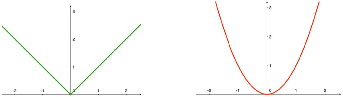
• L1 Loss:
  $$l(\hat{y},y)=|\hat{y}-y|$$
• L2 Loss:
  $$l(\hat{y},y)=(\hat{y}-y{)}^2$$

Classification

• Cross Entroypy Loss ( Negative Log Softmax)
  $$\begin{gathered} H(p,q)=-\sum _{y_i}p(y_i)\log q(y_i)\iff L=H(p,q)=-\log \frac{e^{s_{i^{\ast }}}}{{\Sigma }_j{e}^{s_j}},wherep(y_{i^{\ast }})=1 \\ \sum _{y_i}p(y_i)=1,\sum _{y_i}q(y_i)=1 \end{gathered}$$
  $p(y_i=1)$ is the ground-truth probability of category $i$
  $q(y_i=1)$ is the predicted probability of category $i$

Activation Function (Non-linear)

• Rectified Linear Unit (ReLU):
  $$f(x)=\{\begin{array}{c}0,forx\le 0\\ x,forx>0\end{array}$$
• Exponential Linear Unit (ELU):
  $$f(x)=\{\begin{array}{c}\alpha (e^x)-1,forx\le 0\\ x,forx>0\end{array}$$

Multi-Layer Perceptron (MLP)

• A MLP with activation & $\ge 1$ hidden layers is able to simulate ANY function $f(x)$ where $x$ is the input.
• Back Propagation (Gradient Descent)
• SGD OR Adam (Step Optimizer)

CNN

• Features can be extracted in a local neighborhood.
• VS MLP
  1. Sparse connection vs. Dense
  2. Weight sharing vs. Unique weights
  3. Local invariant vs. Local variant :
     - Features should not depend on the location within the image
     - Make the same prediction no matter where is the object in the image
• Output length $o$
  $$o=\lfloor \frac{n+p-k}{s}\rfloor +1$$
  • kernel size $k$: unknown/trainable parameters
  • Input length $n$: receptive field
  • Padding $p$
  • Stride $s$: Less compute & Increase receptive field

2D-CNN

$$Y_{i,j}=\sum _{a=0}^{k_h-1}\sum _{b=0}^{k_w-1}{X}_{i\ast s_h+a,j\ast s_w+b}\times W_{a,b}$$

• Multiple features $\to$ Multiple kernels & Inputs
  $$Y_{l,i,j}=\sum _{d=0}^{c_i-1}\sum _{a=0}^{k_h-1}\sum _{b=0}^{k_w-1}{X}_{d,i+a,j+b}\times W_{l,d,a,b}+b_l,l\in [0,c_o)$$
• Parameter size $c_o\times k_h\times k_w$
• Output shape $(c_o,o_h,o_w)=(c_o,\lfloor \frac{n_h+p_h-k_h}{s_h}\rfloor +1,\lfloor \frac{n_w+p_w-k_w}{s_w}\rfloor +1)$
• Computation cost $O((c_o\times k_h\times k_w)\times (o_h\times o_w))$

3D-CNN

• Natural extension of 2D Convolution
• Input: Each small cube contains $d$ features/channels
• Kernel: Each small cube contains $d$ weights
• Output: Each small cube is a scalar

Pooling (Matrix$\to$Vector)

• Aggregate information in each receptive field
  • Max
  • Average
• No trainable parameter
• Same padding/stride method

Deep Learning for Point Cloud

• 3D convolution
• Multi-view projection onto images + 2D convolution
• Simply run 1D/2D convolution or even MLP on point cloud (order)

VoxNet (3D convolution)¹

• Content of each grid cell
  • Binary
  • Number of points
  • Probability
  • etc. (TSDF or TDF)
• Accuracy on ModelNet40: 83%
• Conv(o, k, s)
  • o: number of kernels
  • k: size of kernel (same for x/y/z)
  • s: stride (same for x/y/z)

MVCNN (Multi-view)²

Point CNN (MLP)

• Activation function:
  $$h_W,b(x)=f(W^{T}x)=f(\sum _{i=1}^3{w}_i{x}_i+b)=f(w_1{x}_1+w_2{x}_2+w_3{x}_3+b)$$
• Not Permutation Invariant
  $$f(w_1{x}_3+w_2{x}_1+w_3{x}_2+b)\ne h_{W,b}(x)$$

PointNet³

• shared MLP + max pool = PN
• T-Net is a PointNet itself
• Process each point (feature) independently $n\times C_1\to n\times C_2$
• Use Max/Average to pool the features $n\times C\to 1\times C$
  
• Proof – PointNet is able to simulate any function on the point cloud
  $$|f(S)-\gamma (MAX(h(x_1),\cdots ,h(x_n)))|<ϵ$$
  • $\forall ϵ>0,\exists h:{\mathbb{R}}^m\to {\mathbb{R}}^{m^{\prime }},and\gamma :{\mathbb{R}}^n\to \mathbb{R}$, $h\to$ Shared MLP, $\gamma \to$ MLP for global feature
  • Input points S = { x 1 , . . , x n } , x i ∈ R m , x i ∈ [ 0 , 1 ] S=\{x_1,..,x_n\},x_i\in\R^m,x_i\in[0,1] S={x1​,..,xn​},xi​∈Rm,xi​∈[0,1],Denote the space of $S$ as $\chi$, i.e., $S\in \chi$
  • A continuous function $f:\chi \to \mathbb{R}$
  • MAX function: takes $n$ vectors, give element-wise maximum
  • $h(\cdot )$ maps $x_i$ to the some deterministic position of a huge vector, By Voxel Grid Downsampling.
  • MAX$(h(x_1),\cdots ,h(x_n))$ simply builds a voxel grid representation, there will be lots of 0 elements because of empty cells in voxel grid.
  • $\gamma (\cdot )=reconstructthepoints+f(\cdot )$
    
    
• Critical Points Set & Upper Bound Shape
  
  
• Limitations of PointNet
  • CNN has multiple, increasing receptive field
  • PointNet has one receptive field – all points

Voxel Feature Encoding (VFE)

PointNet++

• In each set abstraction:
  • Sampling: FPS
    • Point #: $N_{i-1}\to N_i$
  • Grouping:
    • Radius Neighbors ( + random sampling)
    • K Nearest Neighbors
  • PointNet
    • Point #: $N_i$
    • Channel #: $C_{i-1}\to C_i$
    • Concatenate with coordinates so $d+C_{i-1}\to C_i$
    • Normalize point coordinate in the group
    • Centered with the Node
      
• Multi-scale grouping (MSG)
  • Multiple Grouping & PointNet
    • $r=0.1$ grouping + PN
    • $r=0.2$ grouping + PN
    • $r=0.4$ grouping + PN
    • This is compute intensive
  • Concatenate the multi-scale feature vectors
    
• Multi-resolution grouping (MRG)
  • Get features from previous level (previous previous level)
  • Still increase compute
    
• Interpolation
  • Upsample the features from previous layer
  • $x\in {\mathbb{R}}^3$: point coordinates at the upsampled level, # = $N_1$
  • $f\in {\mathbb{R}}^{C_2}$: interpolated features
  • $x_i\in {\mathbb{R}}^3$: point coordinates at the previous level ($N_2$ points)
  • $w_i\in \mathbb{R}$: reciprocal of distance $d(x,x_i)$
  • $f_i\in R^{C_2}$: point features at the previous level
    $$f^{(j)}(x)=\frac{{\Sigma }_{i=1}^k{w}_i(x)f_i^{(j)}}{{\Sigma }_{i=1}^k{w}_i(x)}where{w}_i(x)=\frac{1}{d(x,x_i{)}^p},j=1,\cdots ,C$$
    
• Data Augmentation
  • Normalization: zero-mean & centered-with-node
  • Input Point Dropout (DP)
  • Gaussian Noise
  • Rotation ( Less overfitting & Worse performance)

---

1. VoxNet: A 3D Convolutional Neural Network for Real-Time Object Recognition, D Maturana, et.al. ↩︎

2. Multi-view Convolutional Neural Networks for 3D Shape Recognition, Hang Su et.al. ↩︎

3. PointNet: Deep Learning on Point Sets for 3D Classification and Segmentation. Cr Qi, et.al., CVPR 2017 ↩︎