【信号处理】基于扩展卡尔曼滤波器和无迹卡尔曼滤波器的窄带信号时变频率估计（Matlab代码实现）

目录

1 概述

2 数学模型 

3 运行结果

4 结论 

5 参考文献

6 Matlab代码实现

---

1 概述

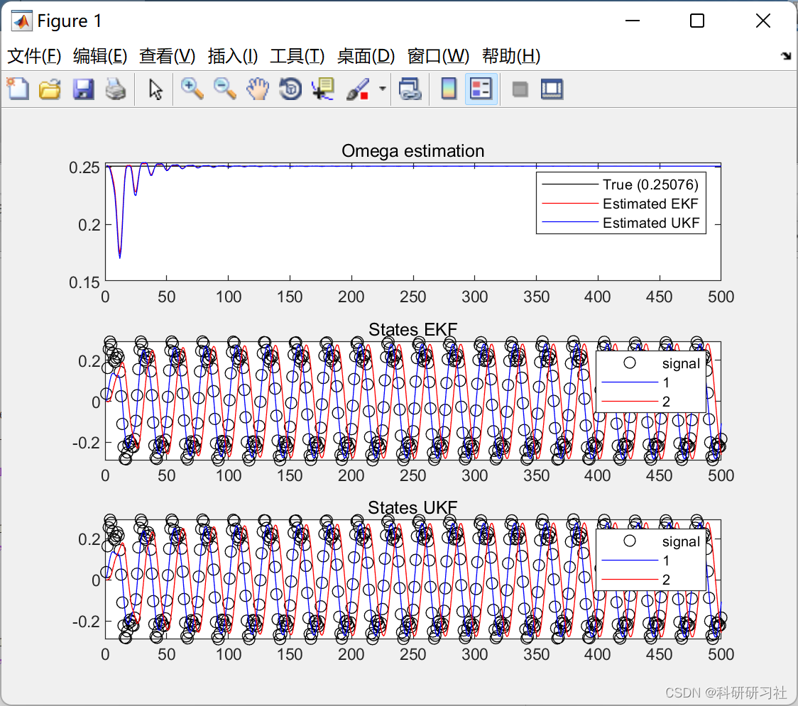
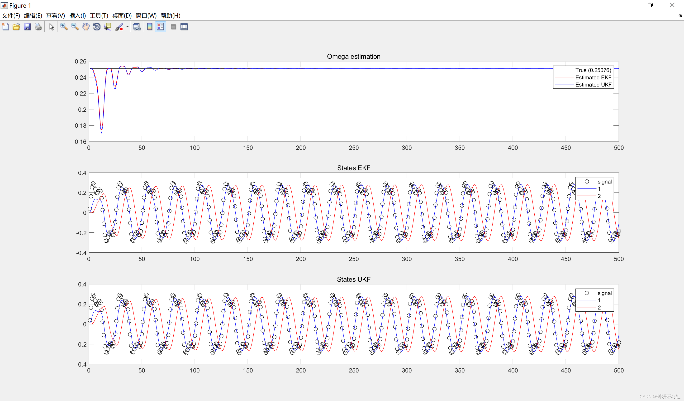
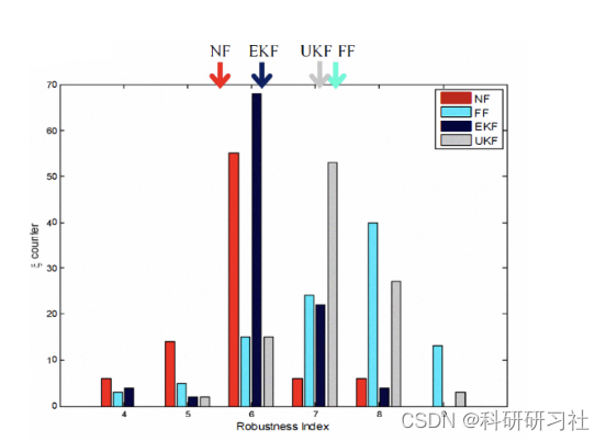
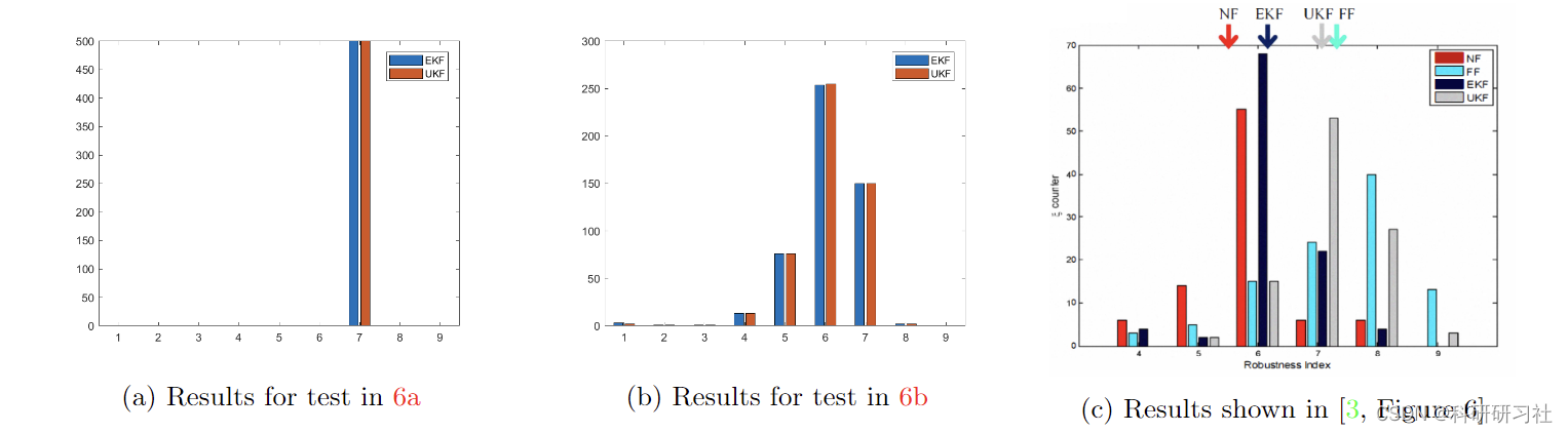
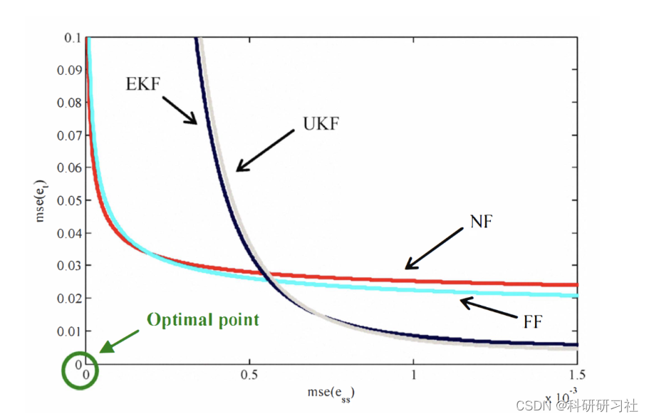
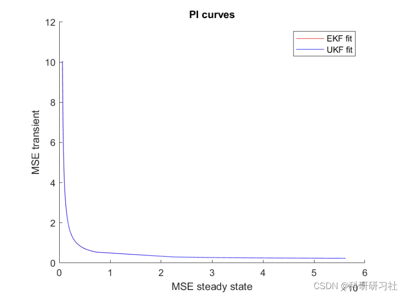
本文讲解和比较了基于卡尔曼滤波器的频率跟踪方法的能力，例如扩展卡尔曼滤波器 (EKF) 和无味卡尔曼滤波器 (UKF)，以跟踪窄带谐波信号的时变频率。这些结果与 Savaresi 等人的结果进行了比较。在 [3] 中。为了评估算法实现的估计质量，使用了两个标准：性能指数 (PI) 和鲁棒性指数 (RI)，如 [3] 中所述。引入了辅助收敛比以更好地解释 PI 图。考虑两个信号：从现实世界记录的单频正弦信号和生成的噪声信号，该信号具有随时间变化的频率，遵循阶跃分布。该算法能够以~10-7 的精度估计真实世界的信号，并实现与 [3] 一致的性能。在最后一节中显示和讨论了获得的结果。

本文讨论了估计嵌入噪声的窄带谐波信号的频率问题；特别是基于卡尔曼滤波器的方法，例如扩展卡尔曼滤波器 (EKF) 和无迹卡尔曼滤波器 (UKF)。为了评估算法实现的估计质量，引入了两个标准：性能指数（PI）和鲁棒性指数（RI），以及辅助收敛比。已对记录的真实信号和生成的噪声信号进行了测试。详细文章见第3部分。

2 数学模型 

所提出的模型是从信号表示为笛卡尔平面中具有角速度 Φ(t) 的旋转矢量构建的。通过将向量沿轴的两个投影和瞬时频率作为状态变量推导出三阶状态空间模型（ARMA 表示）

详细讲解见：

%% RI
clear all
close all
clc
fclose('all');

global logpath;

addpath('./ukf')
addpath('./ekf')
addpath('./generate')
addpath('./ri')

PLOT_PREDICTION = false;
PLOT_PROFILE = false;
COMPUTE = true;

% Parameters
initial_omega = pi/2;
step_profile = [pi/11 -pi/5.5 pi/4 -pi/3.4 pi/2.8 -pi/2.5 pi/2 -pi/1.6 pi/1.4]; % Approximation of Fig.2 on the paper
step_length = 400;    
sigma = 1e+1;
q = 1e-5;
r = sigma*q;
n_simulations = 500;
initialization_noise_sigma = 0.001;
threshold = 120;
% sigma_noise = 2e-2;
% sigma_omega_noise = 1e-3;
sigma_noise = 4e-1;
sigma_omega_noise = 3e-1;

if (PLOT_PREDICTION)
    ri_figure = figure('visible','off');
    set(ri_figure, 'Position', [0, 0, 720, 720],'Resize','off')
end

namestring = sprintf('q%1.2e_s%1.2e_sn%1.2e_sno%1.2e',q,sigma,sigma_noise,sigma_omega_noise);
logpath = strcat(pwd,'\data\ri\',namestring,'\')
if ~exist(logpath,'dir'), mkdir(logpath), end

if (COMPUTE)
    ri_ekf = zeros(1,n_simulations);
    ri_ukf = ri_ekf;
    for ii = 1:n_simulations
        fprintf('***** Iteration %d *****\n',ii)
        % Generate signal
        [signal, omega]=generate_signal_step(step_length,initial_omega,step_profile,sigma_noise,sigma_omega_noise);

        %% Track    
        x_pred_0 = [0, 0, normrnd(omega(1),omega(1)*initialization_noise_sigma)]; % Initialization

        pred_vec_ekf = ekf( ... 
            signal, ...%signal
            x_pred_0, ...%x_pred_0
            initialization_noise_sigma, ...%sigma_init
            r, ... %r,
            q ... %q
        );
        pred_vec_ukf = ukf( ... 
            signal, ...%signal
            x_pred_0, ...%x_pred_0
            initialization_noise_sigma, ...%sigma_init
            r, ... %r,
            q ... %q
        );

        % Take only the state we are interested in
        pred_omega_ekf = pred_vec_ekf(3,:); 
        pred_omega_ukf = pred_vec_ukf(3,:); 

        disp('************ EKF *************');
        ri_ekf(ii) = compute_ri(pred_omega_ekf,omega,step_length,threshold);
        disp('************ UKF *************');
        ri_ukf(ii) = compute_ri(pred_omega_ukf,omega,step_length,threshold);

        % Plot ground truth and predictions
        if PLOT_PREDICTION
            set(0, 'currentfigure', ri_figure);
            clf;
            title('Predictions for RI');
            t = 1:length(omega);
            stairs(t, omega, 'k');
            xlabel('Samples')
            ylabel('Omega')
            set(gca,'YLim',[0,pi]);
            set(gca,'YTick',0:pi/4:pi);
            set(gca,'YTickLabel',{'0' 'pi/4','pi/2','3/4pi','pi'});
            hold on
            plot(t,pred_omega_ekf,'ro');
            plot(t,pred_omega_ukf,'bx');
            legend('True','EKF','UKF')
            RI(ii) = getframe;
        end
    end
    
    if (PLOT_PREDICTION)
        generate_video(strcat('ri_',namestring),RI);
    end

    save(strcat(logpath,'ri_ekf.mat'),'ri_ekf')
    save(strcat(logpath,'ri_ukf.mat'),'ri_ukf')
else
    if exist('ri_ekf.mat','file') && exist('ri_ukf.mat','file')
        load(strcat(logpath,'ri_ekf.mat'),'ri_ekf')
        load(strcat(logpath,'ri_ukf.mat'),'ri_ukf')
    else
        error('No saved curves. Recompute.')
    end
end

n_steps = length(step_profile);
steps_axis = 1:n_steps;
psi_ekf = hist(ri_ekf, steps_axis);
psi_ukf = hist(ri_ukf, steps_axis);

if PLOT_PROFILE 
    figure(1)
    hold off
    stairs(omega)
    xlabel('Samples')
    ylabel('Omega')
    set(gca,'YLim',[initial_omega-pi/2,initial_omega+pi/2]);
    set(gca,'YTick',0:pi/4:pi);
    set(gca,'YTickLabel',{'0' 'pi/4','pi/2','3/4pi','pi'});
end

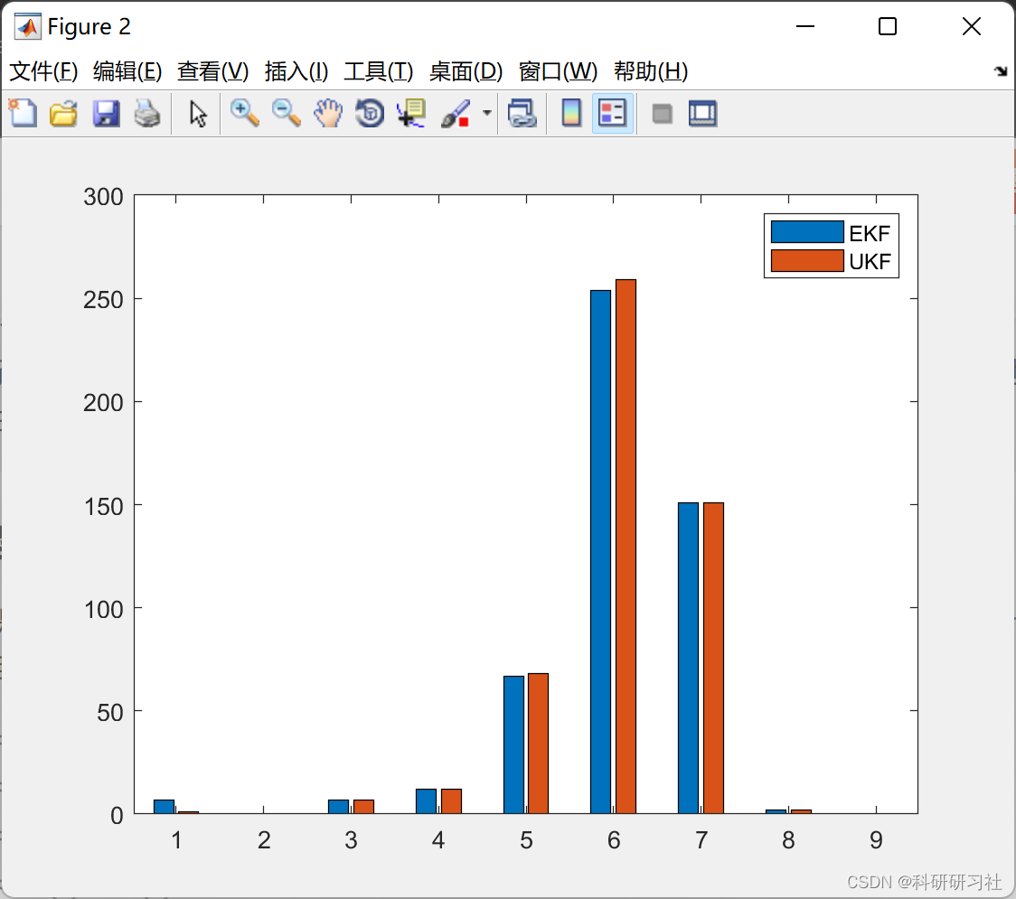
ri_figure = figure(2);
title('RI')
bar(steps_axis,[psi_ekf', psi_ukf'])
legend('EKF','UKF')
saveas(ri_figure, strcat(logpath,'ri_figure_',namestring,'.png'), 'png');

3 运行结果

  

   

4 结论 

本文讨论了估计嵌入噪声的窄带谐波信号的频率问题；特别是基于卡尔曼滤波器的方法，例如扩展卡尔曼滤波器 (EKF) 和无迹卡尔曼滤波器 (UKF)。为了评估算法实现的估计质量，引入了两个标准：性能指数（PI）和鲁棒性指数（RI），以及辅助收敛比。已对记录的真实世界信号和生成的噪声信号进行了测试。剩余详细文章见第3部分。

部分理论引用网络文献，如有侵权请联系博主删除。

5 参考文献

[1] Corbetta S ,  Dardanelli A ,  Boniolo I , et al. Frequency estimation of narrow band signals in Gaussian noise via Unscented Kalman Filter[C]// Proceedings of the 49th IEEE Conference on Decision and Control, CDC 2010, December 15-17, 2010, Atlanta, Georgia, USA. IEEE, 2010.

[2] Dash P K ,  Hasan S ,  Panigrahi B K . Adaptive complex unscented Kalman filter for frequency estimation of time-varying signals[J]. Iet Science Measurement Technology, 2010, 4(2):93-103.

[3] S. Bittanti and S. Savaresi. “On the Parameterization and Design of an
Extended Kalman Filter Frequency Tracker”. In: IEEE transactions on
automatic control 45.9 (2000), pp. 1718–1724.
[4] B. Boashash. “Estimating and Interpreting the instantaneous frequency of
a signal”. In: Proceedings of the IEEE 80.4 (1992), pp. 540–568.
[5] S. Savaresi et al. “Frequency estimation of narrow band signals in Gaussian
noise via Unscented Kalman Filter”. In: 49th IEEE Conference on Decision
and Control (2010), pp. 2869–2874.

6 Matlab代码实现