【状态估计】基于PMU的多回路配电系统状态估计（Matlab代码实现）

👨‍🎓个人主页：研学社的博客 

💥💥💞💞欢迎来到本博客❤️❤️💥💥

🏆博主优势：🌞🌞🌞博客内容尽量做到思维缜密，逻辑清晰，为了方便读者。

⛳️座右铭：行百里者，半于九十。

📋📋📋本文目录如下：🎁🎁🎁

目录

💥1 概述

📚2 运行结果

🎉3 文献来源

🌈4 Matlab代码、数据、文章讲解

---

💥1 概述

文献来源：

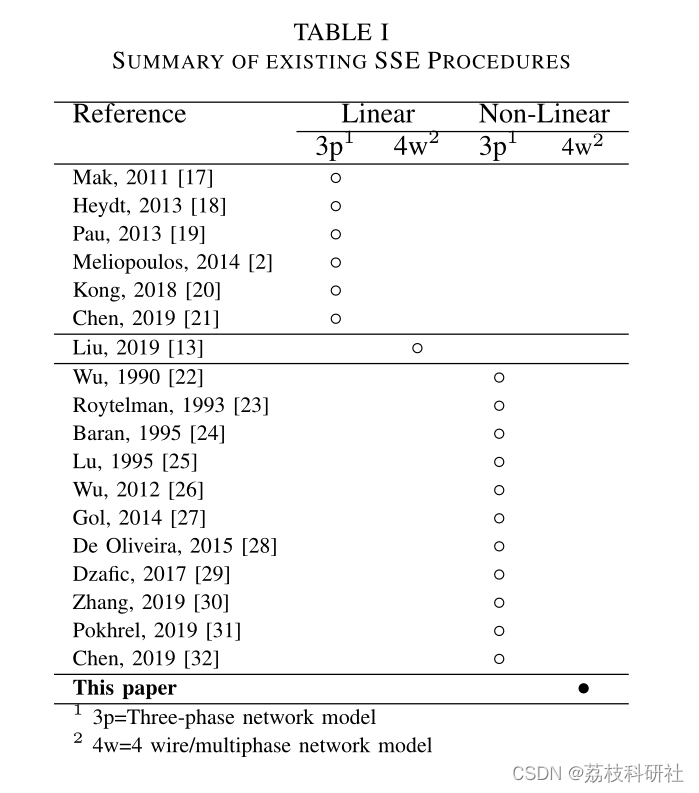
 线性网络建模和相量测量单元（PMU）简化了传统的系统状态估计（SSE）问题。现有的基于多相SSE PMU的模型是线性的，包括作为固定不变参数的接地电阻。然而，接地电阻很大程度上取决于湿度和温度随时间的变化。因此，在不平衡运行情况下，时变中性点接地电压（NEV）可能高于城市地区允许的接触电压和跨步电压。接地电阻现在可以使用专用仪表进行监测，因此可以作为测量和状态变量适当地纳入多重SSE问题中。因此，SSE问题变得非线性，标准线性解方法不再适用。这一事实在文献中被忽视了。为了填补研究空白，提出了一种基于多接地SSE PMU的新公式。作为一项关键贡献，线性SSE方法中使用的正态方程结构被扩展为非线性方程结构，以便能够估计接地电阻、中性点对地电压和中性点电流。为了说明目的，将该建议应用于2总线示例中，并在大规模条件下成功应用并与现有方法进行了比较。

系统状态估计是未来电力系统的基石[1]。状态估计器可以提供一个适当的数学框架，用于根据输配电系统组件的模型验证现场测量

当前趋势表明，基于功率测量的传统系统状态估计器（SSE）可以逐渐被使用相量测量单元（PMU）同步电流和电压变量的估计器所取代。三相域中加权最小二乘（WLS）状态估计问题的解决方案很简单，因为得到的数学模型是线性的[2]。

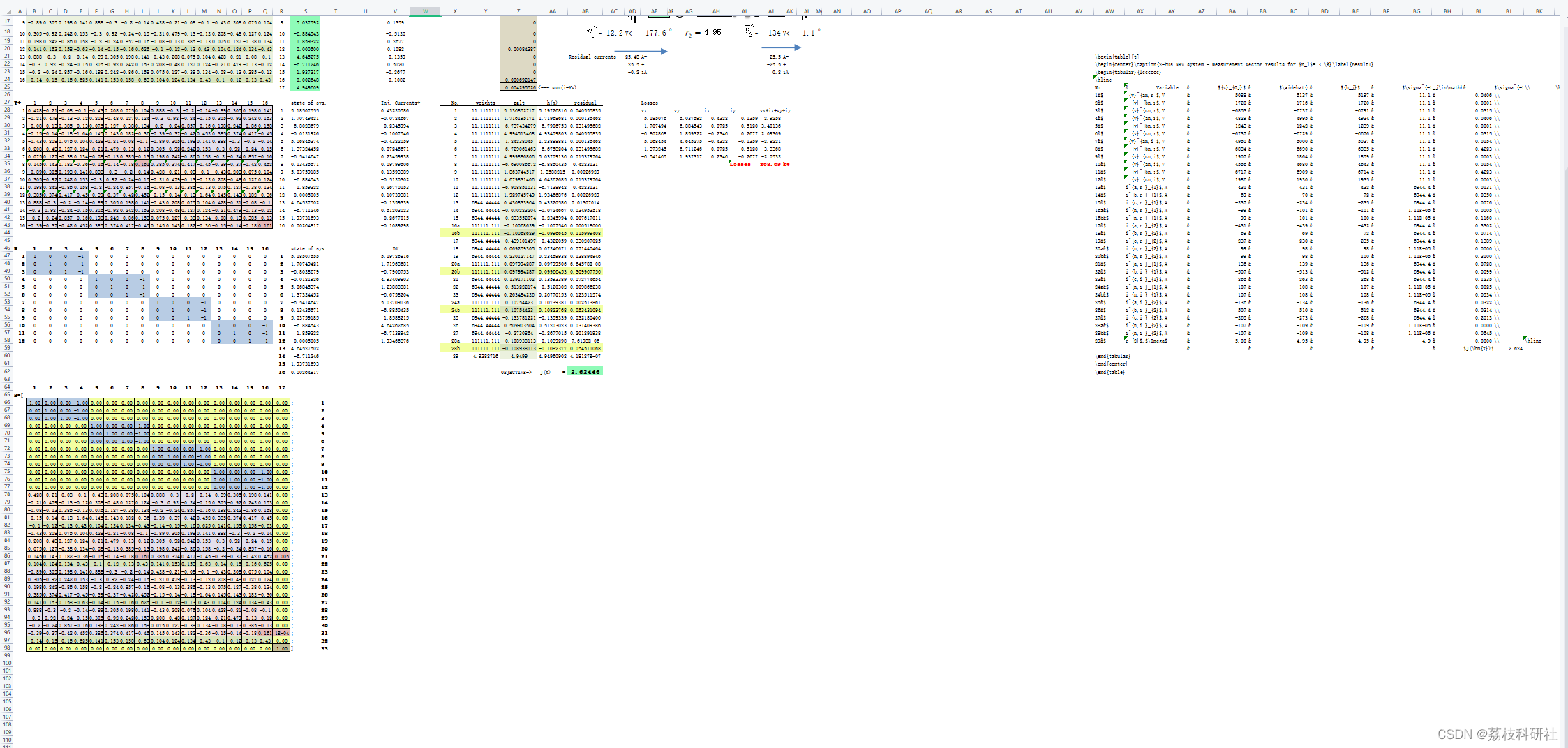
📚2 运行结果

 数据：

部分代码：

%To compile this prograM: mcc -m PMUWLSDSSE.m -o PMUWLSDSSE
clear all
close all
clc
 
%% General parameters
layer=1;%number of layers
nl=.03;%noise level .03=3%
econv=10^-4; %convergence criteria
%% To get 2-bus IEEE Paper Resuls set layer=1
%    layer=1;
%% Runs the  4-wire Power Flow for each layer
[zm,LossesPm,Ym,Ynewm,Ynew2m,rm,injectm,vm,SLm]=KerstingGeneric_powerflow(layer);
zx{layer}=num2cell(zm);
LossesPmx{layer}=num2cell(LossesPm);
Ymx{layer}=num2cell(Ym);
Ynewx{layer}=num2cell(Ynewm);
Ynew2x{layer}=num2cell(Ynew2m);
rx{layer}=num2cell(rm);
injectmx{layer}=num2cell(injectm);
vmx{layer}=num2cell(vm);
SLmx{layer}=num2cell(SLm);

%% Begins the iterative process
nb=2^layer;
z0=cell2mat(zx{layer});
LossesP=cell2mat(LossesPmx{layer});
Y=cell2mat(Ymx{layer});
Ynew=cell2mat(Ynewx{layer});
Ynew2=cell2mat(Ynew2x{layer});
r=cell2mat(rx{layer});
inject=cell2mat(injectmx{layer});
v=cell2mat(vmx{layer});
SL=cell2mat(SLmx{layer});
%% 
ustat=length(Y)+nb-1;% State Vars
m=length(z0);% number of measurements
%% Noise generator, altering the OpenDSS solution zm
lowerbound=-1;
upperbound=1;
for j=1:m
        zalt(j,1)=z0(j,1)*(1+nl*(-lowerbound+(lowerbound+upperbound)*rand(1,1))); 
        %zalt(j,1)=z0(j,1)*(1+nl*unifrnd(lowerbound,upperbound)); 
        %zalt(j,1)=z0(j,1)*(1+nl*normrnd(lowerbound,upperbound));         
end
if layer==1
% Only for l=1 and nl=3% - Paper example
   zalt=[5.13685271701070;1.71619517122123;-6.73743427864737;4.99451346817954;1.24238044981855;-6.72906146331143;4.99988680620950;-6.6900866719488;1.86374451728886;4.67983140587769;-6.90885103136665;1.92974574908040;0.430833963684793;-0.0702232038049941;-0.233552074214137;-0.100686290465729;-0.439101497362902;0.0692593051264286;0.230127146593019;0.0979942874546346;0.139171102396880;-0.513222174262098;0.263484226235493;0.107544229788664;-0.133781221303544;0.509903503818708;-0.273085400259189;-0.108938112961564;4.94990000000000;-0.100686290465729;0.0979942874546346;0.107544229788664;-0.108938112961564];
end
kk=0;
for k=4:4:8*nb
    kk=kk+1;
zalt(m+kk)=zalt(6*nb+k);
end
%% Meter data accuracy and weights calculation
sigma0=.03;%acuraccy of the meters
SIGMAv0=sigma0*10; %Accuracy (dev stad 1*sigma0% on a scale 10000V)
SIGMAi0=sigma0*.400; %Accuracy (dev stad 1*sigma0% on a scale 400A)
SIGMAin0=sigma0*.100; %Accuracy (dev stad 1*sigma0% on a scale 100A)
SIGMAz0=3*sigma0*5; %Accuracy (dev stad 3*sigma0% on a scale 5 ohm)
SigV=ones(1,6*(nb))*SIGMAv0^-2;
SigI=[];
for i=1:nb 
SigI=horzcat(ones(1,3)*SIGMAi0^-2,ones(1,1)*SIGMAin0^-2, ones(1,3)*SIGMAi0^-2,ones(1,1)*SIGMAin0^-2,SigI);
end
SigZ=ones(1,nb-1)*SIGMAz0^-2;
We=horzcat(SigV,SigI,SigZ);
for k=1:2*nb
We(m+k)=SIGMAin0^-2;
end
W=diag(We);
WL=horzcat(SigV,SigI,SigZ)';
%% Build h(x) and H(x) matrix (Outside de while loop, only constant parameters
Ox=zeros(3,4);
A=[1 0 0 -1;0 1 0 -1;0 0 1 -1];
for k1=1:2*nb
    for k2=1:2*nb
   M{k1,k2}=Ox; 
    end
end   
for k=1:2*nb
   M{k,k}=A; 
end
M2=cell2mat(M);
[m2c,m2w]=size(M2);
%Jacobian precalculation
H=zeros(m+2*nb,ustat);
Yone=zeros(nb-1,nb*8);
H=vertcat(M2,Ynew,Yone,Ynew2);
jj=0;
for k=m-nb+2:m
  jj=jj+1;
  H(k,length(v)+jj)=1;
 end
e=1;iteration=1;
%% 4-Wire Distrinution System State Estimation Procedure
while e>econv   
% calculate h(x) Non linear elements
h1=M2*v;
h2=Ynew*v;
kk=0;
for  k=8:4:4*nb
kk=kk+1;
h2(k)=h2(k)-inv(r(kk))*v(k,1);
h2(k+4*nb)=h2(k+4*nb)-inv(r(kk))*v(k+4*nb,1);
end
h3=eye(nb-1)*r;
h4=Ynew2*v;
h=[h1',h2',h3',h4']';
%% Update the Jacobian with non-linear elements
j1=0;
 for k=m2c+8:4:m2c+nb*4
    j1=j1+1;  
    H(k,4+4*j1)=H(k,4+4*j1)-inv(r(j1));
 end
 j2=0;
 for k=m2c+4*nb+8:4:m2c+nb*8
  j2=j2+1;    
   H(k,4+4*nb+4*j2)=H(k,4+4*nb+4*j2)-inv(r(j2));
 end
  j3=0;
 for k3=m2c+8:4:m2c+nb*4
  j3=j3+1;    
   H(k3,8*nb+j3)=v(k3-m2c,1)*(r(j3))^(-2);
  end 
  j4=0;
 for k4=m2c+4*nb+8:4:m2c+nb*8
  j4=j4+1;    
   H(k4,8*nb+j4)=v(k4-m2c,1)*(r(j4))^(-2);
  end
%% Two matrices!
 Bs=H'*diag(We);
 Gs=Bs*H;
 isposdef = all(eig(Gs)) > 0;%is Gs positive definite?
 %% Inverse as a function of Bs and Gs
  time0=cputime;
R = chol(Gs)';%Choelsky decomposition L'*L=Gs
t=Bs*(h-zalt);
u(1)=0;%Forward substitution
flag=0;
 for i=1:ustat  
 u(i)=inv(R(i,i))*(t(i)-flag);
 flag=0;
 if i<ustat
 for j=1:i   
 flag=R(i+1,j)*u(j)+flag; 
 end
 end
 end
 dx(ustat,1)=0;%backward substitution
 flag=0;
 for i=ustat:-1.0:1
 dx(i,1)=inv(R(i,i))*(u(i)-flag);
 flag=0;
 if i>1
  for j=ustat:-1:i 
  flag=R(j,i-1)*dx(j,1)+flag; 
  end
 end
 end
  time(iteration)=cputime-time0;
% time3=cputime;
% dx=-inv(H'*W*H)*H'*W*(zalt-h); %Direct without Cholesky
% time4(iter)=cputime-time3
x=vertcat(v,r);
x=x-dx;
for k=1:8*nb
v(k,1)=x(k);
end
for k=1:nb-1
r(k,1)=x(k+8*nb);
end
iteration=iteration+1;
e=max(abs(dx));
%% End of the DSSE
end
%% Key performance indexes
InverseTime=mean(time)% Gain matrix factorization time
ConvergenceTime=sum(time)% Gain matrix factorization time
IterNumber=iteration%number of iteration to reach convergence
J=(zalt-h)'*W*(zalt-h) %Residual
Confidence=J-chi2inv(.01,m-ustat);
pValue =1-chi2cdf(J,m-ustat)%Confidence level >.99% not suspicious bad data
% Estimated active power losses
for k=1:4*nb;
vc(k,1)=complex(v(k),v(k+4*nb)) ;  
 vcm(k,1)=complex(vm(k),vm(k+4*nb)) ;  
end
for k=1:8*nb
ij(k,1)=h(k+6*nb);  
end
for k=1:4*nb
ijc(k,1)=complex(ij(k),ij(k+4*nb)) ;  
end
P=real(vc).*real(ijc)+imag(vc).*imag(ijc);
LossesPe=sum(P);
%% Verify i=[Y].v and i=^[Y*].v
sum(ij-Ym*v);
kk=0;
for k=8:4:4*nb
    kk=kk+1;
Ynew(k,k)=Ynew(k,k)-inv(r(kk));
end
kk=0;
for k=4*nb+8:4:8*nb
        kk=kk+1;
Ynew(k,k)=Ynew(k,k)-inv(r(kk));
end
sum(ij-Ynew*v);

🎉3 文献来源

部分理论来源于网络，如有侵权请联系删除。

[1]P. M. De Oliveira-De Jesus, N. A. Rodriguez, D. F. Celeita and G. A. Ramos, "PMU-Based System State Estimation for Multigrounded Distribution Systems," in IEEE Transactions on Power Systems, vol. 36, no. 2, pp. 1071-1081, March 2021, doi: 10.1109/TPWRS.2020.3017543.

🌈4 Matlab代码、数据、文章讲解