


👨🎓个人主页:研学社的博客
💥💥💞💞欢迎来到本博客❤️❤️💥💥
🏆博主优势:🌞🌞🌞博客内容尽量做到思维缜密,逻辑清晰,为了方便读者。
⛳️座右铭:行百里者,半于九十。
📋📋📋本文目录如下:🎁🎁🎁
目录

💥1 概述
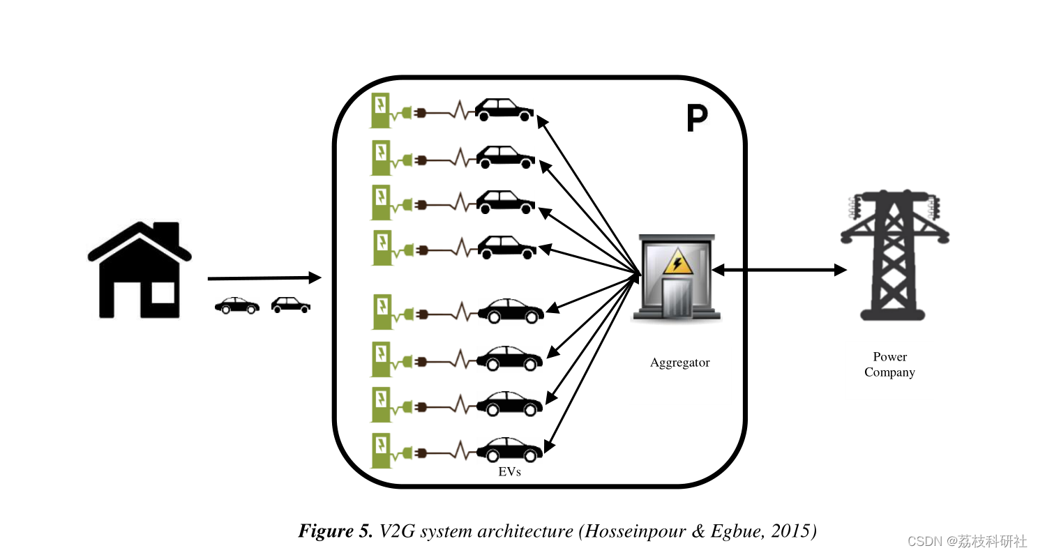
V2G优化调度:
设计了一种算法,以充电成本最小的方式安排500辆电动汽车使用一个充电站,同时随机安排任意少数电动汽车前往指定的房屋负载,在那里放电并返回充电站。模拟测试了三种不同的场景,第一,客户满意度(即电动汽车车主满意度)被认为是放电所赚的钱与充电所花的钱之间的总差额,第二,客户满意度与第一种场景相同,但在模拟结束时减去未完成的费用的总成本,第三,客户满意度考虑了放电的利润,充电的成本,在整个模拟过程中,未完成充电的总成本和从每辆电动汽车切换的成本。
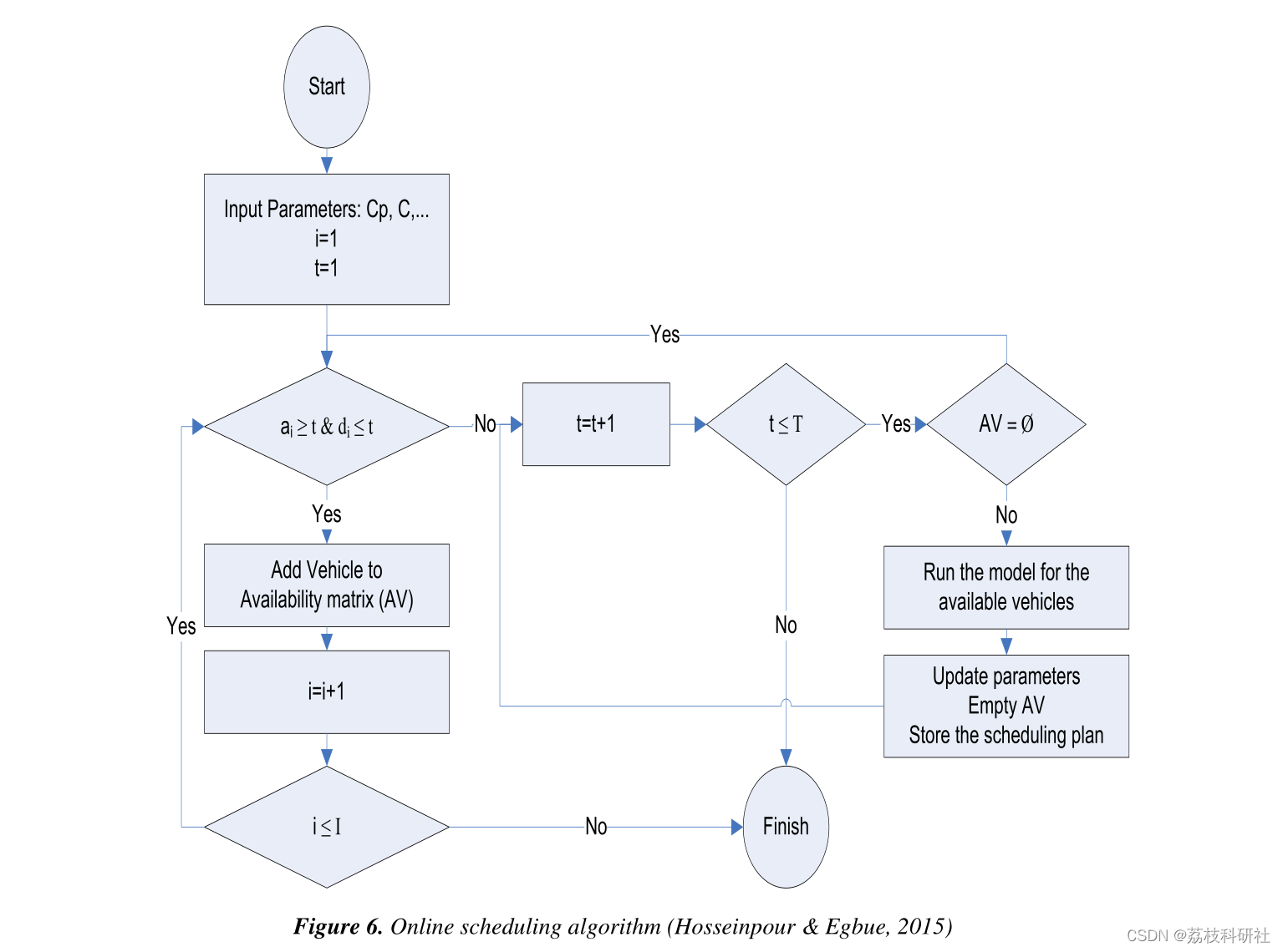
为了模拟电动汽车的行为,使用了许多不同的基于时间的变量。以下是最关键的变量,是决定客户满意度的主要因素:a) X -充电状态(1或0)b) Y -放电状态(1或0)c) SOC -充电状态(以最大电池容量的百分比测量)与变量一起,电动汽车初始化的值包括最大电池容量,第三种情况的最大开关数量等。在整个仿真过程中的每个时间单位,对x和y变量以及能量约束实施各种系统约束,以确保稳定性和车辆到电网系统的工作。例如,单个EV在单个单位时间内只能在不行驶时处于充电或放电状态,而不能同时处于充电或放电状态(即x = 1或y = 1,不能同时处于充电或放电状态)。
另一个关键的系统要求是充电站有足够的能量来继续为正在充电的车辆充电。在第三种情况中引入了一个额外的约束,其中每辆电动汽车必须保持在从充电到放电、从充电到空闲等状态允许的最大开关数量限制内。初始化值、EV变量和各种约束方程的基础是Shima Hosseinpour和Ona Egbue的研究论文——优化电动汽车充放电的动态调度。
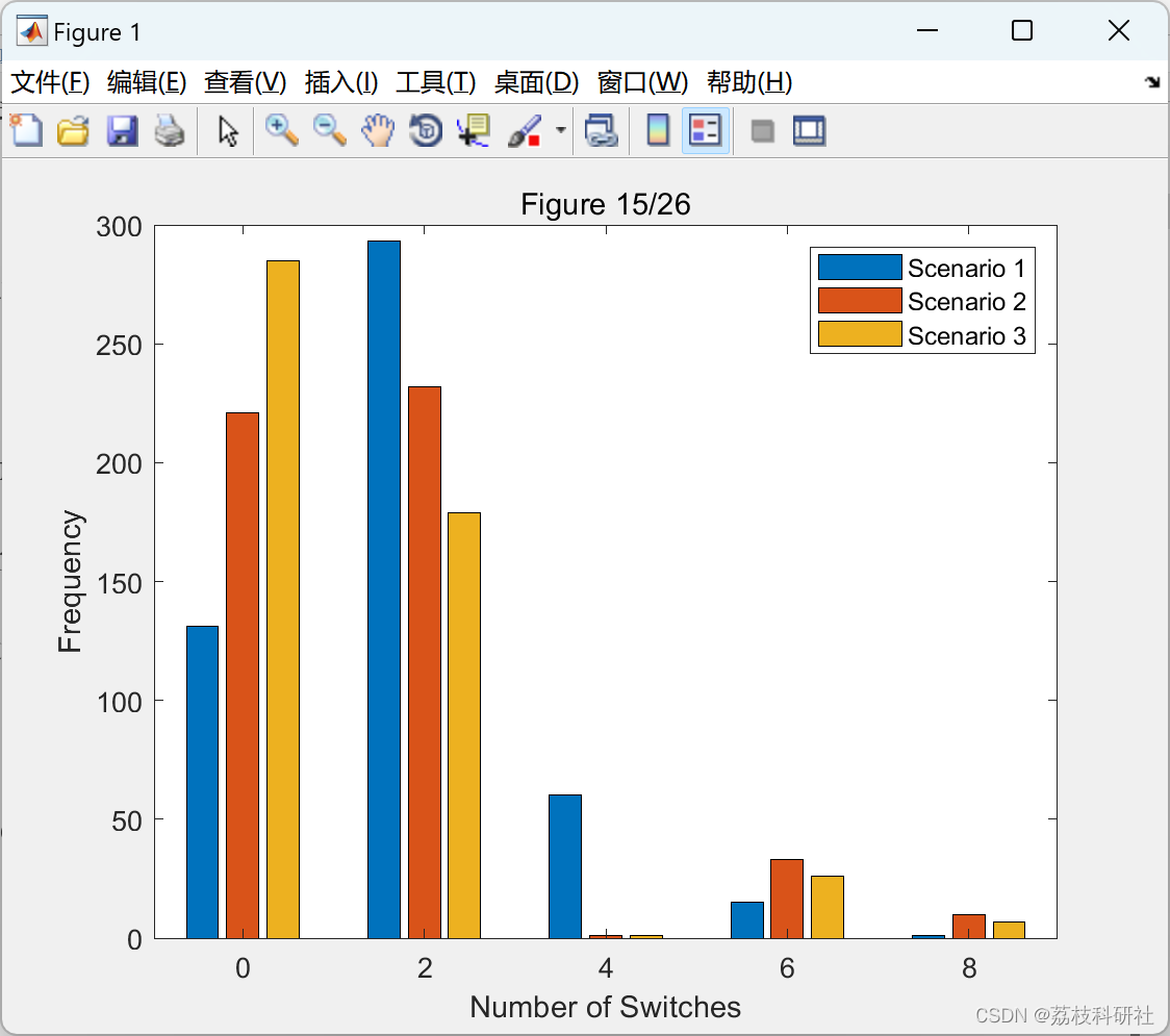
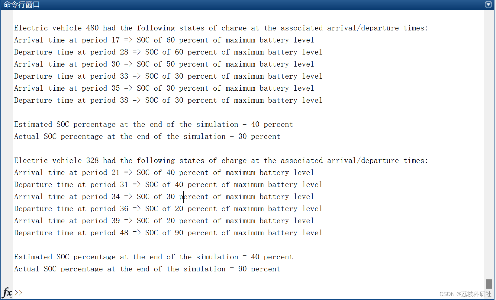
一旦模拟完成,将进行中期模拟行程的车辆的最终充电状态与到达房屋负载时和在房屋负载完成放电后的充电状态进行比较。还制作了各种图形和条形图-每辆电动汽车的开关数量,随机电动汽车的充电状态与时间,在指定房屋进行模拟中期放电行程的电动汽车的充电状态与距离等。
在离线和在线充放电调度模型中,分别开发了三种不同的场景。在第一种场景中,目标函数只考虑电动汽车车主的放电收益和充电成本。因此,该模型预计会对电动汽车进行调度,使它们放电的次数多于充电的次数。在第二个场景中,考虑未完成的充电请求以及放电的利润。因此,未充电电力的惩罚成本被添加到第二种情况的目标函数中。在第三种情况下,根据电池寿命,考虑到电动汽车电池可以拥有的最大开关数量的限制。这个限制包含在模型的约束中。所以,第三种情况的目标函数和第二种情况是一样的。
详细文章讲解及数学模型讲解见第4部分

📚2 运行结果


部分代码:
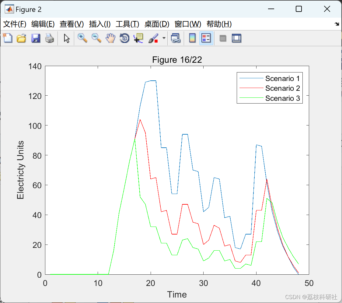
%% Figure 16/22
figure(2)
plot(planning_periods, total_x_1st, planning_periods, total_x_2nd, 'r', planning_periods, total_x_3rd, 'g')
title('Figure 16/22')
xlabel('Time')
ylabel('Electricty Units')
legend('Scenario 1','Scenario 2', 'Scenario 3')
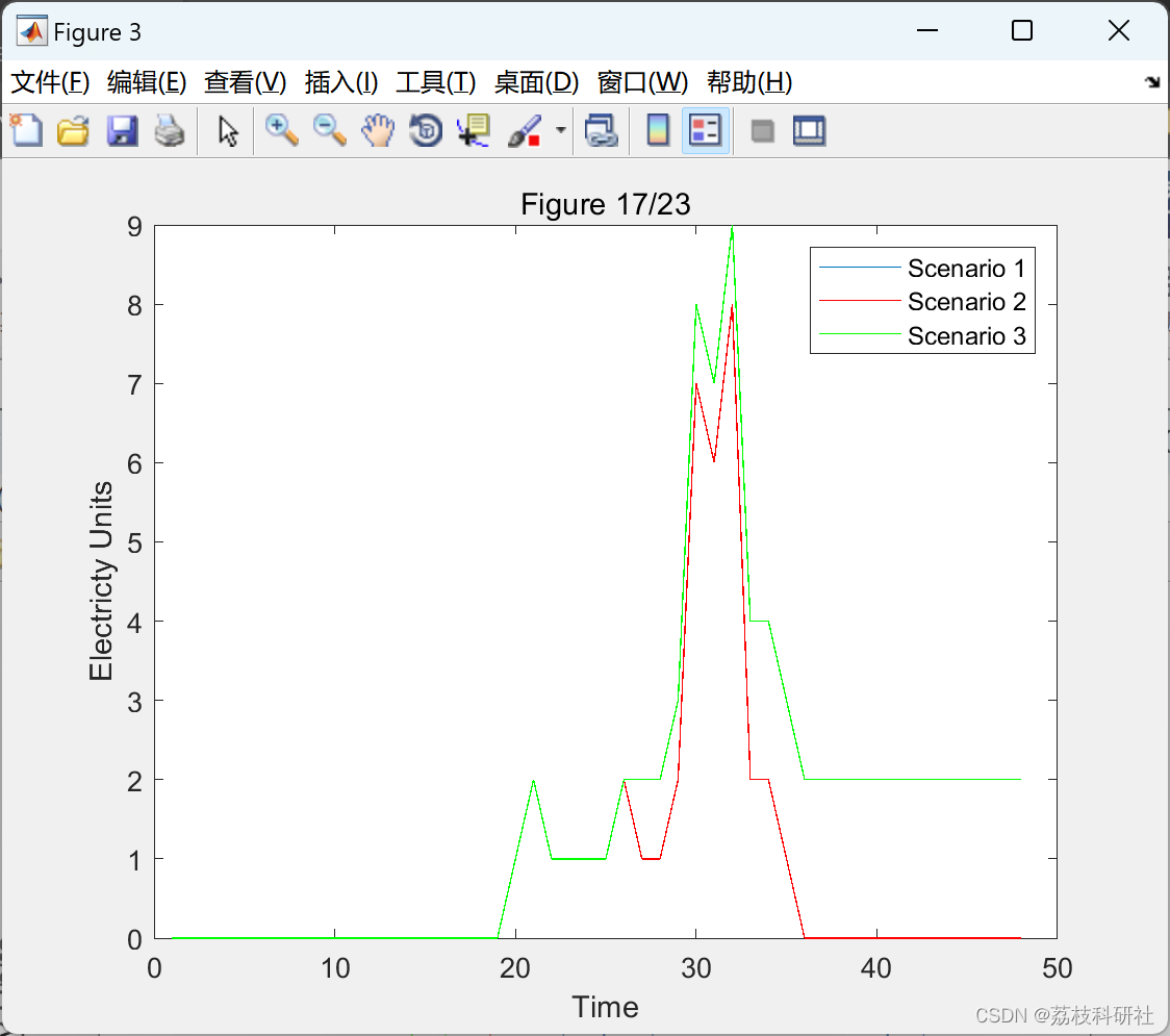
%% Figure 17/23
figure(3)
plot(planning_periods, total_y_1st, planning_periods, total_y_2nd, 'r', planning_periods, total_y_3rd, 'g')
title('Figure 17/23')
xlabel('Time')
ylabel('Electricty Units')
legend('Scenario 1','Scenario 2', 'Scenario 3')
%% Figure 18/27
figure(4)
yyaxis left
plot(planning_periods, total_x_3rd, planning_periods, total_y_3rd)
title('Figure 18/27')
xlabel('Time')
ylabel('Electricity Units')
yyaxis right
plot(planning_periods, Ct_available_EU)
ylabel('Price (cents)')
legend('Charging','Discharging','Price')
%% Figure 19/24
[list_of_total_z_1st, z_index_1st] = sort(list_of_total_z_1st);
z_freq_temp_1st = frequency_of_z_1st;
for i = 1:length(z_freq_temp_1st)
frequency_of_z_1st(i) = z_freq_temp_1st(z_index_1st(i));
if ~ismember(list_of_total_z_1st(i),list_of_total_z_2nd)
list_of_total_z_2nd = [list_of_total_z_2nd list_of_total_z_1st(i)];
frequency_of_z_2nd = [frequency_of_z_2nd 0];
end
if ~ismember(list_of_total_z_1st(i),list_of_total_z_3rd)
list_of_total_z_3rd = [list_of_total_z_3rd list_of_total_z_1st(i)];
frequency_of_z_3rd = [frequency_of_z_3rd 0];
end
end
[list_of_total_z_2nd, z_index_2nd] = sort(list_of_total_z_2nd);
z_freq_temp_2nd = frequency_of_z_2nd;
for i = 1:length(z_freq_temp_2nd)
frequency_of_z_2nd(i) = z_freq_temp_2nd(z_index_2nd(i));
end
[list_of_total_z_3rd, z_index_3rd] = sort(list_of_total_z_3rd);
z_freq_temp_3rd = frequency_of_z_3rd;
for i = 1:length(z_freq_temp_3rd)
frequency_of_z_3rd(i) = z_freq_temp_3rd(z_index_3rd(i));
end
plot_param = zeros(length(frequency_of_z_1st),3);
for i = 1:length(frequency_of_z_1st)
for j = 1:3
if j == 1
plot_param(i,j) = frequency_of_z_1st(i);
elseif j == 2
plot_param(i,j) = frequency_of_z_2nd(i);
else
plot_param(i,j) = frequency_of_z_3rd(i);
end
end
end
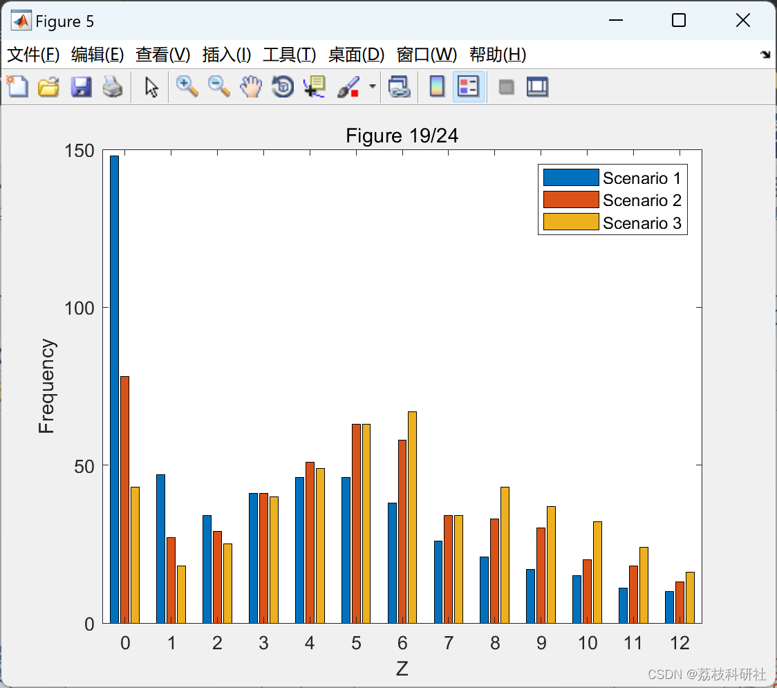
figure(5)
bar(list_of_total_z_1st, plot_param)
title('Figure 19/24')
xlabel('Z')
ylabel('Frequency')
legend('Scenario 1','Scenario 2', 'Scenario 3')
%% Figure 20/25
z_values_1st = [];
z_values_2nd = [];
z_values_3rd = [];
EVs = [];
for i = 1:N
z_values_1st = [z_values_1st EV_1st(i).z];
z_values_2nd = [z_values_2nd EV_2nd(i).z(periods)];
z_values_3rd = [z_values_3rd EV_3rd(i).z(periods)];
EVs = [EVs i];
end
figure(6)
plot(EVs, z_values_1st, EVs, z_values_2nd, 'r', EVs, z_values_3rd, 'g')
xlabel('EV Number')
ylabel('Electricity Units')
title('Figure 20/25')
legend('Z1','Z2','Z3')
%% Figure 21/28
figure(7)
plot(planning_periods, total_x_3rd, planning_periods, cpt_available_EU)
title('Figure 18/27')
xlabel('Time')
ylabel('Electricity Units')
legend('Charging','Capacity')
%% SOC vs distance plot of test EV taking home trip
%Assuming an initial SOC of 100% (i.e., of either 10 EU or 15 EU) can cover
%400 miles at full charge. First determine whether the test EV is PHEV or
%BEV
distance_per_EU = [];
distance_per_period = [];
total_periods = [];
home_vehicle_IDs = [];
for i = 1:N
if ismember(i,home_vehicles)
distance_per_EU = [distance_per_EU 400/EV(i).mc]; %Distance covered per EU depending on the type
distance_per_period = distance_per_EU; %Assume 1 EU is spent in one period of travelling
total_periods = [total_periods EV(i).travel_time];
home_vehicle_IDs = [home_vehicle_IDs i];
end
end
%EV energy vs distance plot
random_num = randi(length(total_periods));
total_periods_vector = zeros(1,total_periods(random_num));
count = 0;
for i = 1:total_periods(random_num)
count = count + 1;
total_periods_vector(i) = count*distance_per_period(random_num);
end
%Create a uniformly distributed distance vector
total_periods_vector = linspace(total_periods_vector(1),total_periods_vector(length(total_periods_vector)),total_periods(random_num)+1);
start_time = EV_1st(home_vehicle_IDs(random_num)).schedule(2);
end_time = EV_1st(home_vehicle_IDs(random_num)).schedule(3);
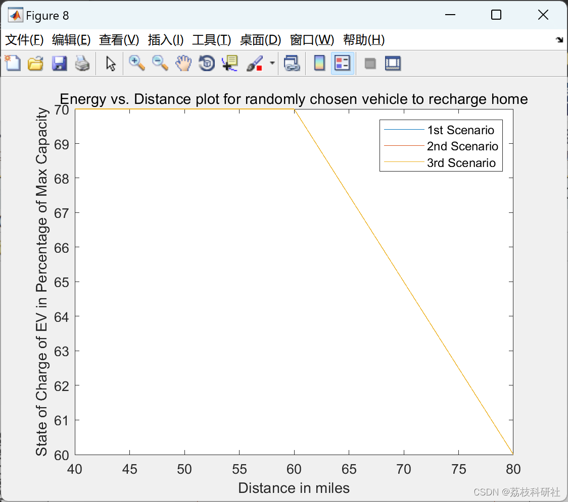
figure(8)
plot(total_periods_vector, EV_1st(home_vehicle_IDs(random_num)).soc(start_time:end_time).*(100.*(EV_1st(home_vehicle_IDs(random_num)).mc).^(-1)),total_periods_vector, EV_2nd(home_vehicle_IDs(random_num)).soc(start_time:end_time).*(100.*(EV_2nd(home_vehicle_IDs(random_num)).mc).^(-1)),total_periods_vector, EV_3rd(home_vehicle_IDs(random_num)).soc(start_time:end_time).*(100.*(EV_3rd(home_vehicle_IDs(random_num)).mc).^(-1)))
title('Energy vs. Distance plot for randomly chosen vehicle to recharge home')
xlabel('Distance in miles')
ylabel('State of Charge of EV in Percentage of Max Capacity')
legend('1st Scenario','2nd Scenario', '3rd Scenario')
figure(9)
plot(total_periods_vector, EV_1st(home_vehicle_IDs(random_num)).soc(start_time:end_time).*(100.*(EV_1st(home_vehicle_IDs(random_num)).mc).^(-1)),total_periods_vector, EV_2nd(home_vehicle_IDs(random_num)).soc(start_time:end_time).*(100.*(EV_2nd(home_vehicle_IDs(random_num)).mc).^(-1)))
title('Energy vs. Distance plot for randomly chosen vehicle to recharge home')
xlabel('Distance in miles')
ylabel('State of Charge of EV in Percentage of Max Capacity')
legend('1st Scenario','2nd Scenario')
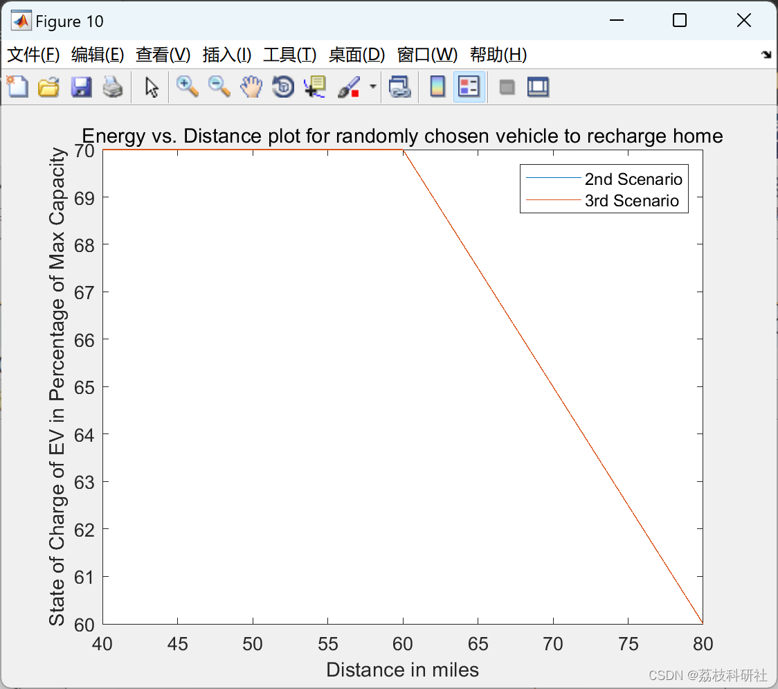
figure(10)
plot(total_periods_vector, EV_2nd(home_vehicle_IDs(random_num)).soc(start_time:end_time).*(100.*(EV_2nd(home_vehicle_IDs(random_num)).mc).^(-1)),total_periods_vector, EV_3rd(home_vehicle_IDs(random_num)).soc(start_time:end_time).*(100.*(EV_3rd(home_vehicle_IDs(random_num)).mc).^(-1)))
title('Energy vs. Distance plot for randomly chosen vehicle to recharge home')
xlabel('Distance in miles')
ylabel('State of Charge of EV in Percentage of Max Capacity')
legend('2nd Scenario', '3rd Scenario')
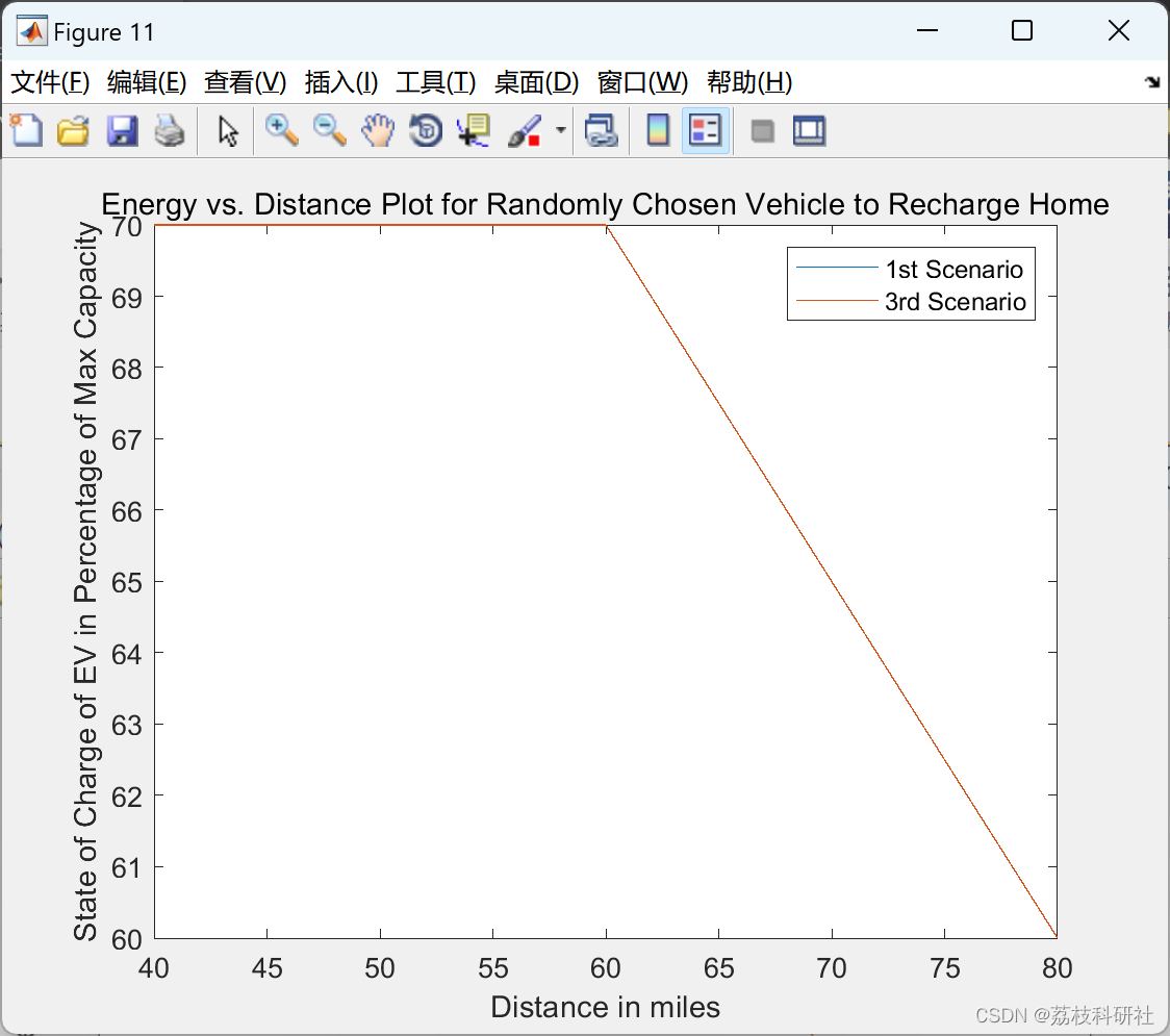
figure(11)
plot(total_periods_vector, EV_1st(home_vehicle_IDs(random_num)).soc(start_time:end_time).*(100.*(EV_1st(home_vehicle_IDs(random_num)).mc).^(-1)),total_periods_vector, EV_3rd(home_vehicle_IDs(random_num)).soc(start_time:end_time).*(100.*(EV_3rd(home_vehicle_IDs(random_num)).mc).^(-1)))
title('Energy vs. Distance Plot for Randomly Chosen Vehicle to Recharge Home')
xlabel('Distance in miles')
ylabel('State of Charge of EV in Percentage of Max Capacity')
legend('1st Scenario', '3rd Scenario')
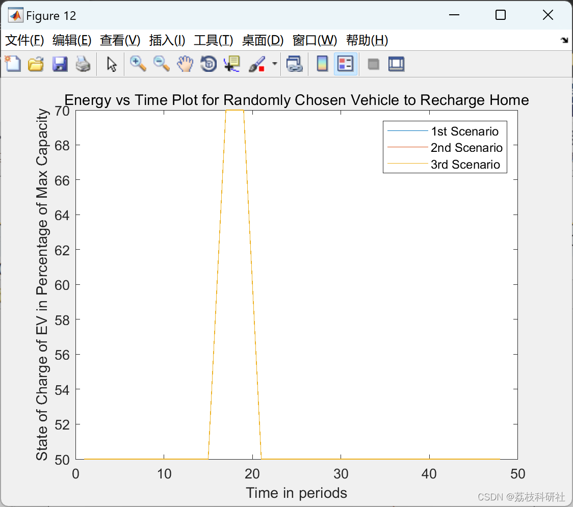
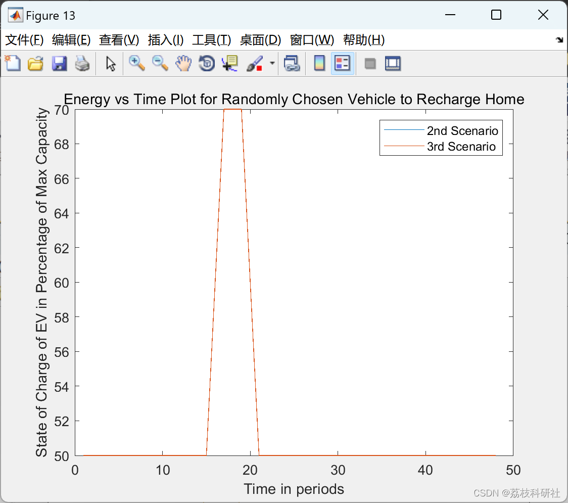
%% SOC vs time plot of test EV taking home trip
figure(12)
plot(planning_periods, EV_1st(home_vehicle_IDs(random_num)).soc.*(100.*(EV_1st(home_vehicle_IDs(random_num)).mc).^(-1)), planning_periods, EV_2nd(home_vehicle_IDs(random_num)).soc.*(100.*(EV_2nd(home_vehicle_IDs(random_num)).mc).^(-1)), planning_periods, EV_3rd(home_vehicle_IDs(random_num)).soc.*(100.*(EV_3rd(home_vehicle_IDs(random_num)).mc).^(-1)))
title('Energy vs Time Plot for Randomly Chosen Vehicle to Recharge Home')
xlabel('Time in periods')
ylabel('State of Charge of EV in Percentage of Max Capacity')
legend('1st Scenario', '2nd Scenario', '3rd Scenario')
🎉3 参考文献
部分理论来源于网络,如有侵权请联系删除。
[1]汪思奇.考虑V2G的区域综合能源系统运行调度优化[J].科学技术创新,2022(34):30-34.
[2]郑鑫,邱泽晶,郭松,廖晖,黄玉萍,雷霆.电动汽车V2G调度优化策略的多指标评估方法[J].新能源进展,2022,10(05):485-494.
[3]肖丽,谢尧平,胡华锋,罗维,朱小虎,刘晓波,宋天斌,李敏.基于V2G的电动汽车充放电双层优化调度策略[J].高压电器,2022,58(05):164-171.DOI:10.13296/j.1001-1609.hva.2022.05.022.


 1328
1328


 被折叠的 条评论
为什么被折叠?
被折叠的 条评论
为什么被折叠?
 到【灌水乐园】发言


