【误差自适应跟踪方法AUV】自适应跟踪（EAT）方法研究（Matlab代码&Simulin实现）

 💥💥💞💞欢迎来到本博客❤️❤️💥💥

🏆博主优势：🌞🌞🌞博客内容尽量做到思维缜密，逻辑清晰，为了方便读者。

⛳️座右铭：行百里者，半于九十。

📋📋📋本文目录如下：🎁🎁🎁

目录

💥1 概述

📚2 运行结果

🎉3 参考文献

🌈4 Matlab代码、Simulink模型、文献

---

💥1 概述

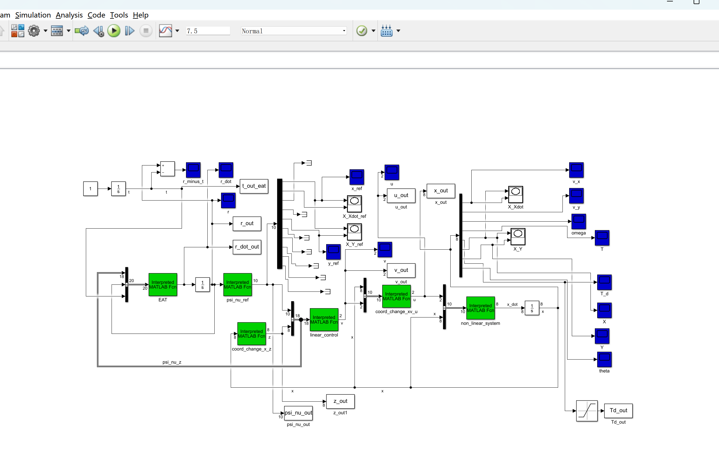
摘要：跟踪问题（即如何遵循先前记忆的路径）是移动机器人中最重要的问题之一。根据机器人状态与路径相关的方式，可以制定几种方法。“轨迹跟踪”是最常见的方法，控制器旨在将机器人移动到移动的目标点，就像在实时伺服系统中一样。对于复杂系统或处于扰动或未建模效应下的系统，如 UAV（无人驾驶飞行器），其他跟踪方法可以提供额外的好处。在本文中，考虑路径描述符参数动态的方法（可称为“误差自适应跟踪”）与轨迹跟踪进行了对比。首先提出了跟踪方法的正式描述，表明两种类型的错误自适应跟踪可以在任何系统中与同一控制器一起使用。仿真实验表明，选择合适的跟踪速率可以提高无人机系统的误差收敛性和鲁棒性。结果表明，误差自适应跟踪方法优于轨迹跟踪方法，产生更快、更鲁棒的收敛跟踪，同时在需要时在实现收敛时保持相同的跟踪速率。

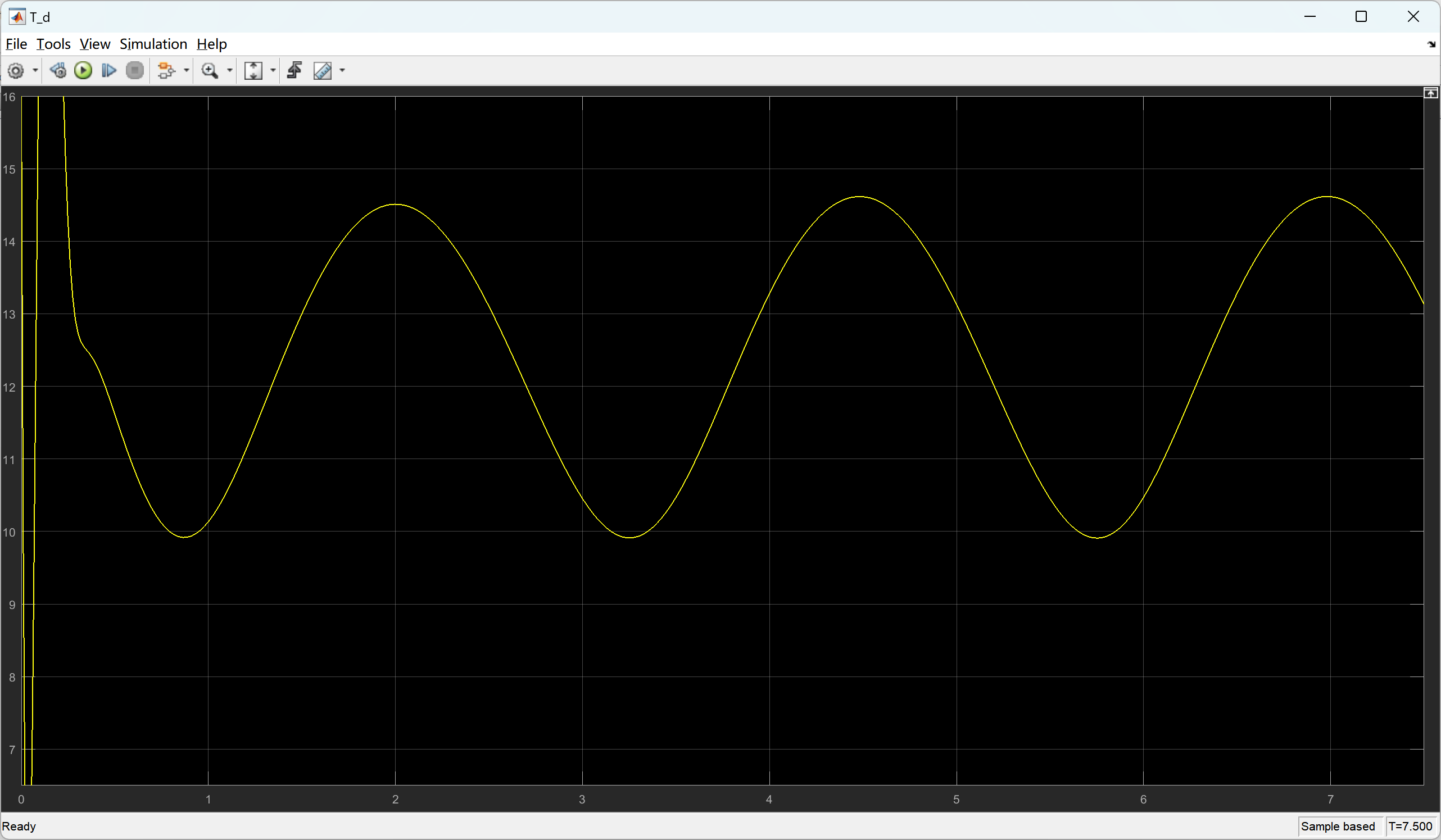
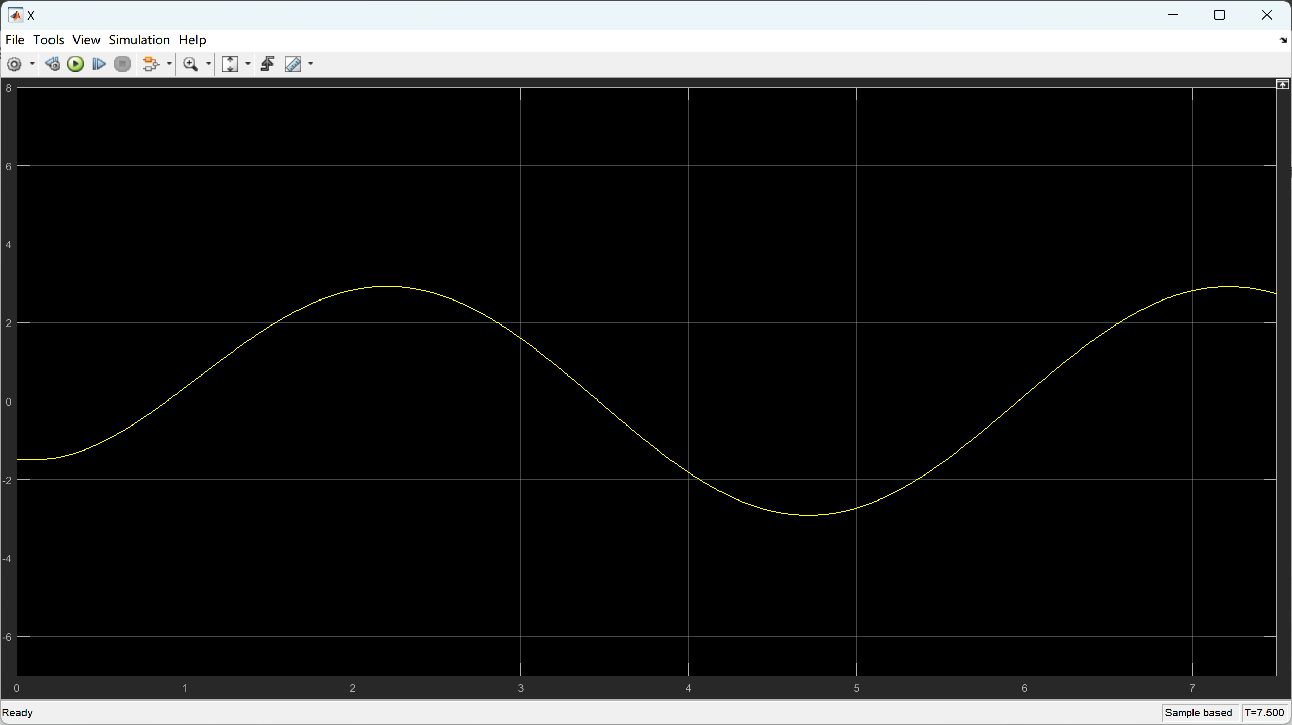
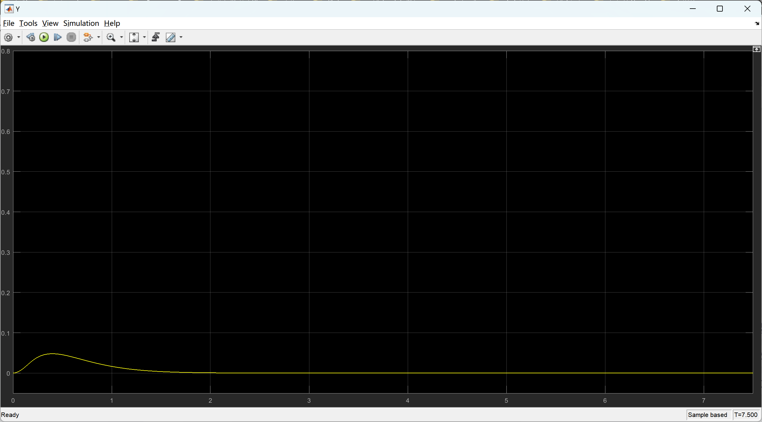
📚2 运行结果

 

 

 

 

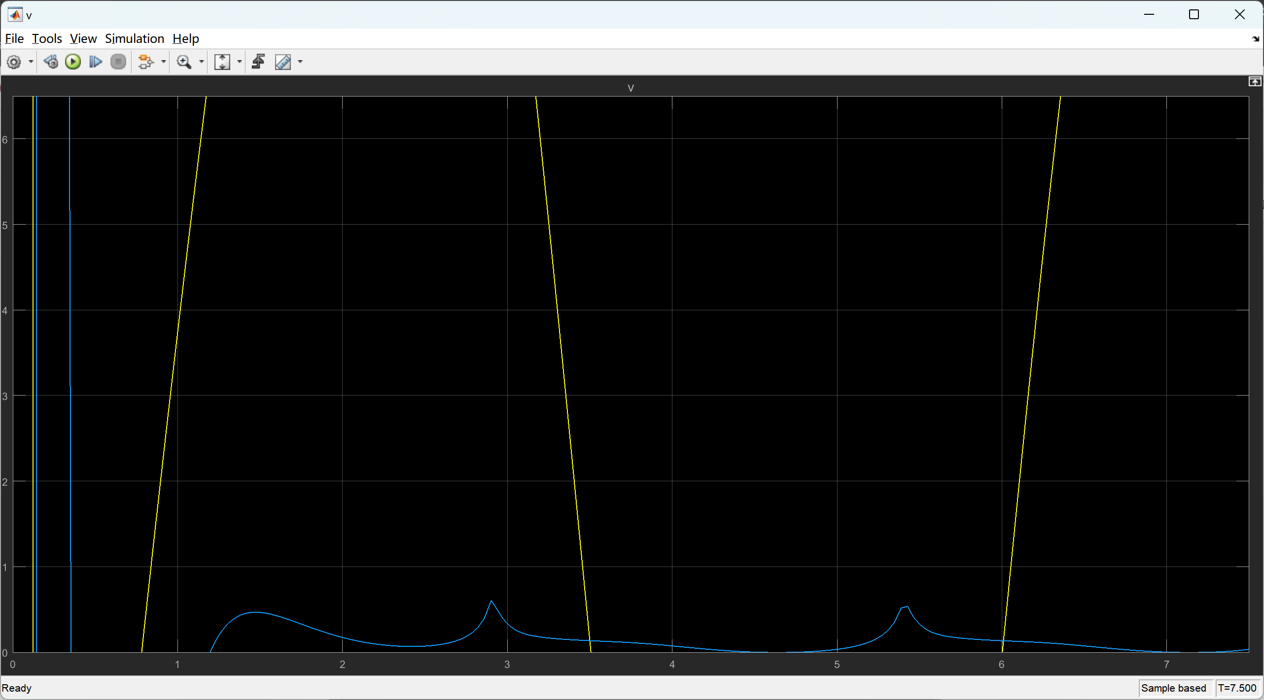
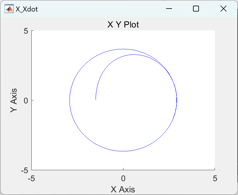
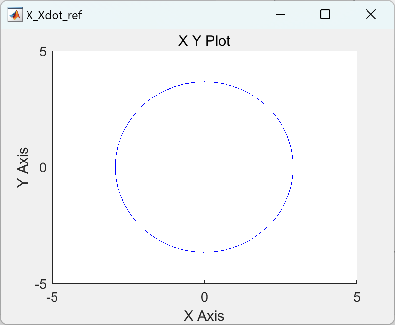
 部分代码：

%% clear 
%% graphic (scope) parameters
% Xmin=-1;
% Xmax= 1;
% Ymin=-1;
% Ymax= 1;
%graphic (scope) parameters
Xmin=-5;
Xmax= 5;
Ymin=-5;
Ymax= 5;
%graphic (scope) parameters
% Xmin=-1;
% Xmax= 7;
% Ymin=-1;
% Ymax= 3.5;

%% Simulation constants
start_time=0;
stop_time=10;

%% system parameters 
pvtol_constants_global;

%% System matrixes
A_0 = [ 0 1 0 0 ; ...
        0 0 1 0 ;...
        0 0 0 1 ;...
        0 0 0 0  ];
A=blkdiag(A_0, A_0);

B_0 = [ 0 ; ...
        0 ;...
        0 ;...
        1 ];
B=blkdiag(B_0, B_0);

%% control matrix according to Hindman/Hauser:
K_0 =[-3604 -2328 -509.25 -39];
K=blkdiag(K_0, K_0);

%% Lyapunov equation
Ac=A+B*K;
Q=eye(8);

global P;
P=lyap(Ac',Q);

%% constants for ref. traj. x_ref(r)=A_ref*sin(w_ref*r)
A_ref=1.857*pi/2;
w_ref=2*pi/5;
%

%% initial condition for x, that is:
% v_x = x_1;
% v_y = x_2; 
% omega = x_3; 
% T   = x_4; 
% T_d  = x_5; 
% 
% x = x_6; 
% y = x_7;
% theta = x_8 ;

% an initial condition not null is necessary for T to prevent div/0 in
% coord_change_xv_u
% initial condition must be concordant  with that of psi_nu. Hence, call to
r_initial=0;
psi_nu_initial = psi_nu_ref(r_initial);

% Hindman/Hauser gave a value of 10.0 for initial Td
% However, analysing the  z(0) values, one gives to 
T_d_initial = 16;% g*m is 10.32
% this other condition gives us a smoother start 
T_initial = 16;% T_d_initial ;

%%%%%%%%%%%%%%%%%%%%%%
%%%%% IDEAL INITIAL CONDITIONS:
%from the coord change x to z, this initial values can be calculated
% remark: using these ideal initial conditions, tracking is perfect!
theta_initial = 0;
omega_initial = -psi_nu_initial(4)*m/T_initial;
%ideal initial conditions:
x_initial = [ psi_nu_initial(2); psi_nu_initial(6); omega_initial; T_initial ; T_d_initial; ...
    psi_nu_initial(1); psi_nu_initial(5); theta_initial ...
    ];  

%%%%%%%%%%%%%%%%%%%%%%
% Hindman/Hauser  uses this initial condition for z(0)
% z_initial = [ -1.5; v_x(0); v_x_dot(0); v_x_dot_dot(0) ; ...
%     0; 0; 0; 0 ...
%     ]
% if the PVTOL were robust, it should be stable against an initial 
% condition like  
%  x_initial = [ 0 ; 0 ; omega_initial ; T_initial ; T_d_initial; ...
%     -1.5 ; 0 ; 0 ...
%     ];  

🎉3 参考文献

部分理论来源于网络，如有侵权请联系删除。

[1]Hauser, J. and Hindman, R. Maneuver regulation from
trajectory tracking: Feedback linearizable systems. 
In Proc. IFAC Symp. Nonlinear Contr. Syst. Design, 638-643. Tahoe City, CA.(1995).

🌈4 Matlab代码、Simulink模型、文献