【R语言】主成分分析

主成成分分析详解

主成分分析经常用于对数据的降维，通过选择具有较高方差的主成分来替代原始的数据。主成分分析的另一个主要用途是解决多重共线性问题。此外，通过仅对所有主成分的子集进行回归，主成分分析可以显著降低基础模型的参数数量。

书上的很少且抽象，不太懂。

看了一个视频有助于理解。直接点击就可以看了

使用R语言进行主成分分析

在进行主成分分析之前，需要判断需要选取多少个主成分。判断的准则很多，包括：
●　根据经验或者理论知识判断主成分个数。
●　根据解释变量方差的积累值的阈值来判断保留的主成分个数。
●　通过变量间的关系矩阵来判断需要保留的主成分个数。
●　基于特征值进行判断，根据Kaiser-Harris准则建议保存特质大于1的主成分。
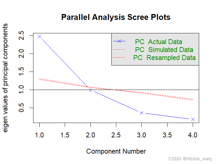
●　使用Cattell碎石图进行判断，碎石图绘制了特征值与主成分数量，这类图可以清晰地展示特征值与主成分个数之间的关系，图形变化最大之前的主成分都可以保留。
●　平行分析法，其原理是模拟一个与原数据集相同大小的矩阵来判断提取的特征值，若真实的某个特征值大于随机数据矩阵的平均特征值，则可以保留。

利用psych包中的fa.parallel( )函数可以对3种准则（特征值大于1、碎石检验、平行分析）进行评价。

> fa.parallel(Thurstone,fa = "pc")
Parallel analysis suggests that the number of factors =  NA  and the number of components =  1 

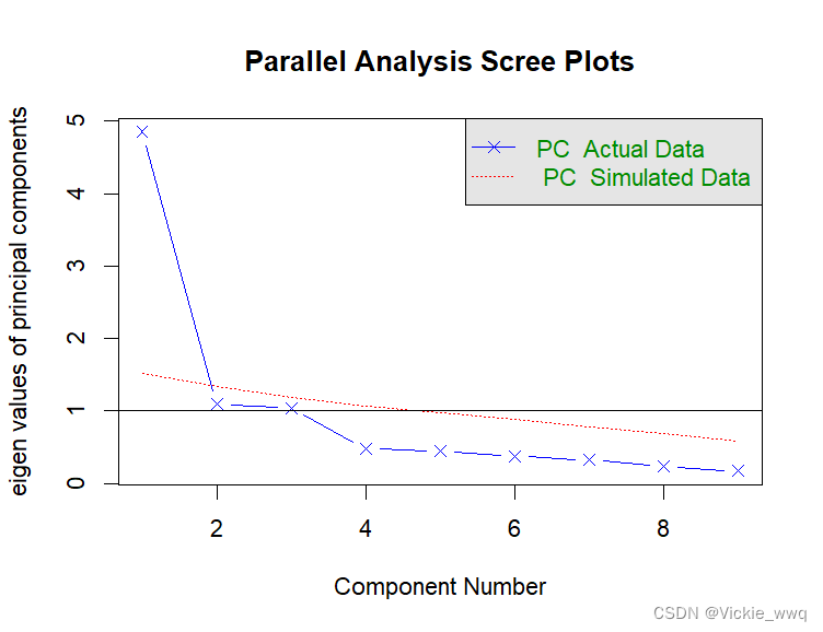
碎石图的结果给出了3种准则的评判结果。
【特征值大于1】特征值大于1的特征包含3个；
【碎石检验】碎石图的曲线从第一个特征到第二个特征之间有急剧的变化，因此，选取第一个主成分；
【平行分析法】有一个特征大于随机矩阵的特征。
总而言之，选取一个主成分最合适。

procomp( )函数
结果得到了所有的主成分，然后根据之前判断的主成分个数，选取相应的主成分，即可得到所需的结果。

> com <- prcomp(Thurstone)
> com
Standard deviations (1, .., p=9):
[1] 4.068067e-01 3.717632e-01 1.747973e-01 1.614655e-01 1.328383e-01 1.137641e-01 8.417453e-02 5.966690e-02 5.116523e-17

Rotation (n x k) = (9 x 9):
                          PC1         PC2        PC3         PC4         PC5          PC6         PC7         PC8         PC9
Sentences         -0.51809588  0.01904674  0.2219406  0.10347521  0.06248519 -0.111471957  0.40722485  0.68008332 0.163013221
Vocabulary        -0.50023933  0.09586015  0.1948562  0.03929555  0.09218721 -0.016188107  0.42092377 -0.71770206 0.004977171
Sent.Completion   -0.51043041  0.05906835  0.1922287  0.05061761 -0.10617941  0.099931122 -0.76715103 -0.04517829 0.290922025
First.Letters      0.17889726  0.41142018  0.2781580 -0.28375796  0.05821963  0.752293096  0.13448197  0.06117109 0.222883485
Four.Letter.Words  0.22201272  0.34066448  0.3832537 -0.47143714 -0.04884194 -0.625099183 -0.02856458 -0.03809150 0.264802257
Suffixes           0.06316668  0.48794084 -0.5349420  0.38650203  0.12836566 -0.114136797  0.06024721 -0.04481668 0.535941908
Letter.Series      0.12799298 -0.46305936  0.1213871 -0.04342013  0.77851211  0.004042136 -0.05517789 -0.05033184 0.375364298
Pedigrees         -0.18269477 -0.36539660 -0.4557516 -0.57758413 -0.32964974  0.079329046  0.14775329 -0.03158129 0.392434091
Letter.Group       0.29283881 -0.34002238  0.3780991  0.44445752 -0.48920364  0.035988647  0.14513339 -0.09806774 0.43224114

psych包的principal( )函数

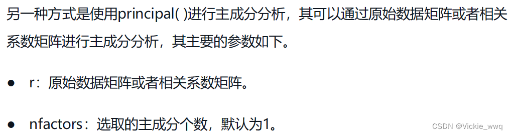
> com <- principal(r = Thurstone,nfactors = 1)
> com
Principal Components Analysis
Call: principal(r = Thurstone, nfactors = 1)
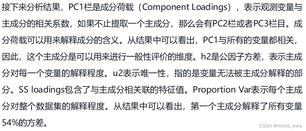
Standardized loadings (pattern matrix) based upon correlation matrix
                   PC1   h2   u2 com
Sentences         0.82 0.67 0.33   1
Vocabulary        0.84 0.70 0.30   1
Sent.Completion   0.80 0.65 0.35   1
First.Letters     0.72 0.52 0.48   1
Four.Letter.Words 0.71 0.51 0.49   1
Suffixes          0.67 0.45 0.55   1
Letter.Series     0.67 0.45 0.55   1
Pedigrees         0.70 0.50 0.50   1
Letter.Group      0.64 0.41 0.59   1

                PC1
SS loadings    4.85
Proportion Var 0.54

Mean item complexity =  1
Test of the hypothesis that 1 component is sufficient.

The root mean square of the residuals (RMSR) is  0.12 

Fit based upon off diagonal values = 0.94

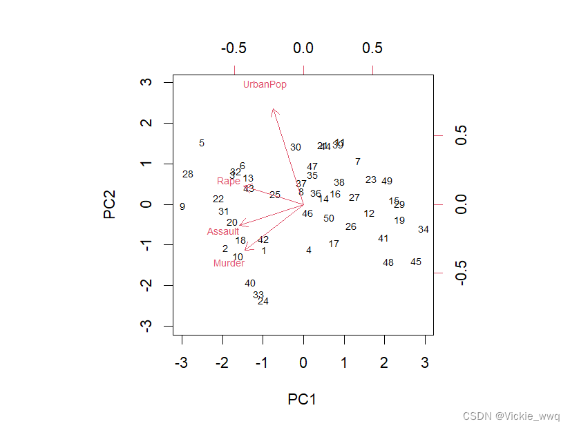
USArrests数据，该数据包括4个连续变量和50条记录。

data("USArrests")
head(USArrests,3)

library(dplyr)
usarrests <- tbl_df(USArrests)
glimpse(usarrests)

apply(USArrests, 2, mean)
apply(USArrests, 2, var)

normalize <- function(x)#编写了一个标准化函数
{
  return((x-mean(x))/sd(x))
}

usarrests2 <- as.data.frame(apply(usarrests, 2, normalize))

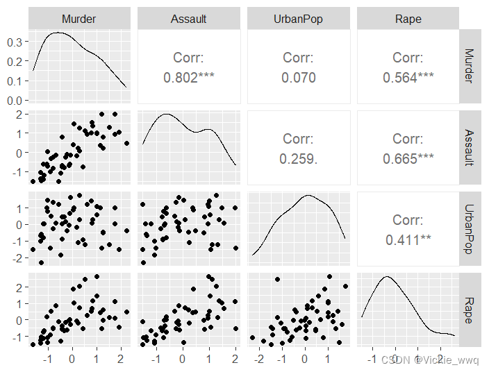
#分析特征的分布及特征之间的相关性
install.packages("GGally")
library(GGally)
ggpairs(data = usarrests2,columns = 1:4,progress = F)

#判断主成分个数
fa.parallel(usarrests2,fa = "pc")
## Parallel analysis suggests that the number of factors =  NA  and the number of components =  1 

#进行主成分分析
pca.out <- prcomp(usarrests2)
pca.out
# Standard deviations (1, .., p=4):
#   [1] 1.5748783 0.9948694 0.5971291 0.4164494
# 
# Rotation (n x k) = (4 x 4):
#   PC1        PC2        PC3         PC4
# Murder   -0.5358995 -0.4181809  0.3412327  0.64922780
# Assault  -0.5831836 -0.1879856  0.2681484 -0.74340748
# UrbanPop -0.2781909  0.8728062  0.3780158  0.13387773
# Rape     -0.5434321  0.1673186 -0.8177779  0.08902432
summary(pca.out)
# Importance of components:
#   PC1    PC2     PC3     PC4
# Standard deviation     1.5749 0.9949 0.59713 0.41645
# Proportion of Variance 0.6201 0.2474 0.08914 0.04336
# Cumulative Proportion  0.6201 0.8675 0.95664 1.00000

biplot(pca.out,scale = 0,cex=0.65)  #绘制双重图