10X单细胞-10X空间转录组联合分析之七----CellDART

hello，大家好，今天再次给大家带来10X单细胞空间联合分析的一个新方法，CellDART，有关10X单细胞空间联合分析的文章呢，其实分享了不少了，在这里列举出来，有需要的可以学习一下

10X单细胞和空间联合分析的方法---cell2location

10X空间转录组和10X单细胞数据联合分析方法汇总

10X单细胞空间联合分析之三----Spotlight

10X单细胞空间联合分析之四----DSTG

10X单细胞空间联合分析之五----spatialDWLS

10X单细胞空间联合分析之六(依据每个spot的细胞数量进行单细胞空间联合分析)----Tangram

方法很多，但是一定要有自己的甄别能力，看看哪个才是适合自己的方法，今天我们分享的方法文献在CellDART: Cell type inference by domain adaptation of single-cell and spatial transcriptomic data，我们今天来看看这个方法有什么特别之处，适合于什么样的数据分析，先来分享文献，最后我们看一下示例代码。

Abstract

Deciphering（澄清，阐明，辨认） the cellular composition in genome-wide spatially resolved transcriptomic data is a critical task to clarify the spatial context of cells in a tissue.（这句话翻译过来就是阐明全基因组空间解析的转录组数据中的细胞组成是阐明组织中细胞空间背景的关键任务，这个确实非常重要），作者这里开发了一个新方法，cellDART, which estimates the spatial distribution of cells defined by single-cell level data using domain adaptation of neural networks(这个东西是什么，需要我们往下看看了) and applied it to the spatial mapping of human lung tissue。The neural network that predicts the cell proportion in a pseudospot, a virtual mixture of cells from single-cell data, is translated to decompose the cell types in each spatial barcoded region（这个是解卷积方法的常规思路）。下面运用这个软件分析了两个数据mouse brain and human dorsolateral prefrontal cortex tissue，当然了，效果不错，老套路了。CellDART is expected to help to elucidate the spatial heterogeneity of cells and their close interactions in various tissues.

Main（Introduction）这里我们总结一下

Breakthrough technologies enabled capturing genome-wide spatial gene expression at a resolution of several cells（10X空间转录组就是这个精度） to the single-cell（单细胞水平的空间转录组还是个大难题） and even subcellular levels（亚细胞水平这个华大好像研发成功了）。
Furthermore, emerging computational approaches facilitated the spatiotemporal tracking of specific cells and elucidated cell-to-cell interactions by preserving the spatial context（这个地方的分析难度相当高）。

• 空间转录组现在唯一的限制因素 一个spot里面包含了多个细胞。尤其a tissue with a high level of heterogeneity, such as cancer, consists of a variety of cells in each small domain of the tissue（这个限制确实影响很大）。Thus, the identification of different cell types in each spot is a crucial task to understand the spatial context of pathophysiology using a spatially resolved transcriptome.
  现在10X空间转录组和10X单细胞联合分析的方法主要有两派，一派是找锚点映射的方法，典型如Seurat，scanpy，另外一种就是解卷积的方法，典型如SPOTlight，cell2location，解卷积的方法占大多数，在解卷积的方法中，calculating the proportion of cell types defined by scRNA-seq data from spots of spatially resolved transcriptomic data can be considered a domain adaptation task（区域适应任务，这个翻译有点土，不过意思还是解卷积那种思路）。A model that predicts cell fractions from the gene expression profile of a group of cells can be transferred to predict the spatial cell-type distribution.（单细胞空间联合分析确实很重要）。

In this paper, we suggest a method, CellDART, that implements adversarial discriminative domain adaptation (ADDA)（这个不知道怎么翻译，需要看看下文理解一下这个意思） to infer the cell fraction in spatial transcriptomic data.从scRNA-seq数据中随机选择的细胞构成一个SPOT，其中细胞的比例是已知的。从SPOT的基因表达中提取细胞成分的神经网络模型适用于存在空间转录组数据的不同domian。 （神经网络模型不知道大家了解多少，涉及到机器学习的知识）。Consequently, the joint analysis of spatial and single-cell transcriptomic data elucidates the spatial cell composition and unveils the spatial heterogeneity of the cells，然后运用这个方法来实际操作一下。

Result 我们首先来看看这个软件的效果

1、Decomposition of spatial cell distribution with CellDART in human and mouse brain data

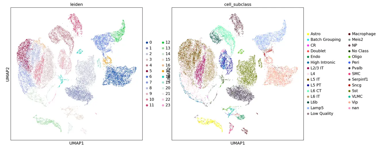
两个示例数据，human dorsolateral prefrontal cortex，mouse brain看一看注释数据

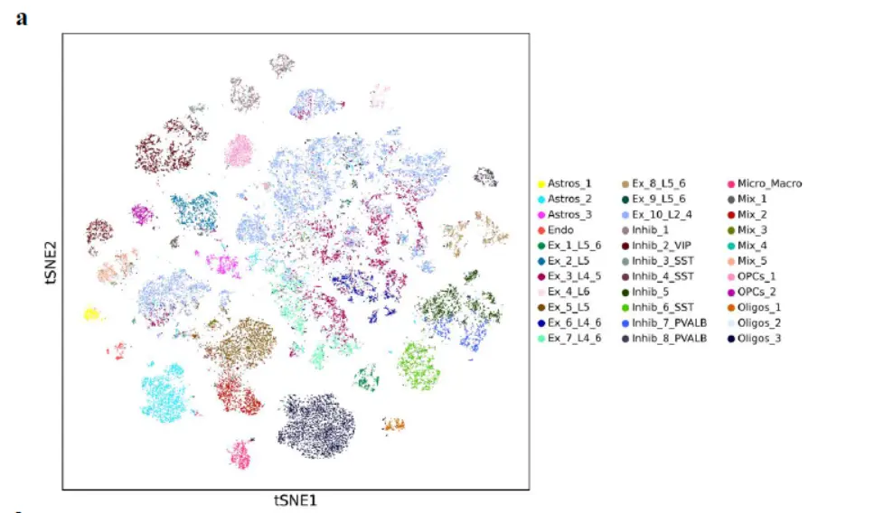
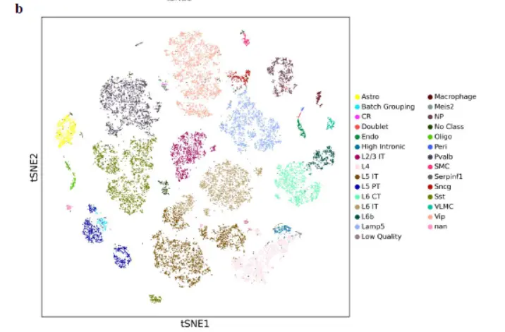
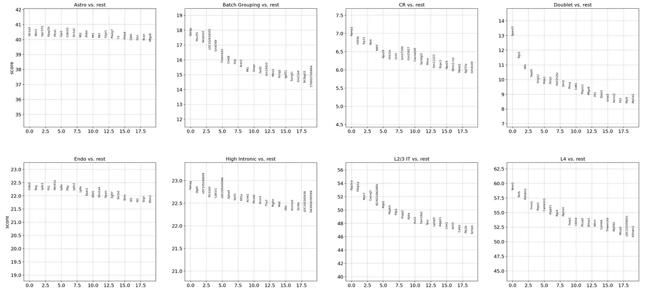
然后是marker gene（感觉并不是很特异）

The cell clusters showed distinct gene expression patterns represented by cell type-specific marker genes。

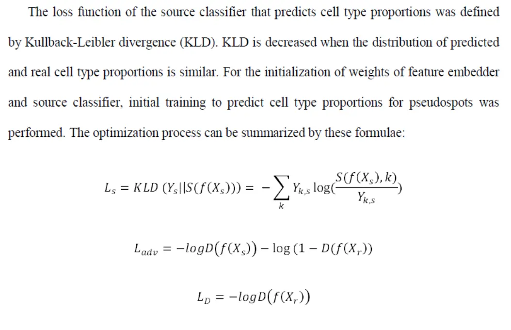
第一步 这里构建伪SPOTA specific number of cells (k = 8) were randomly sampled from the single-cell data with random weights to generate pseudospots(number of pseudospots = 20000)，（8个细胞）。

第二步 composite gene expression values were computed based on marker genes

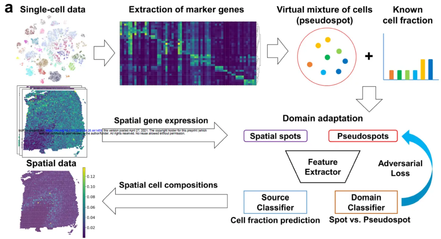
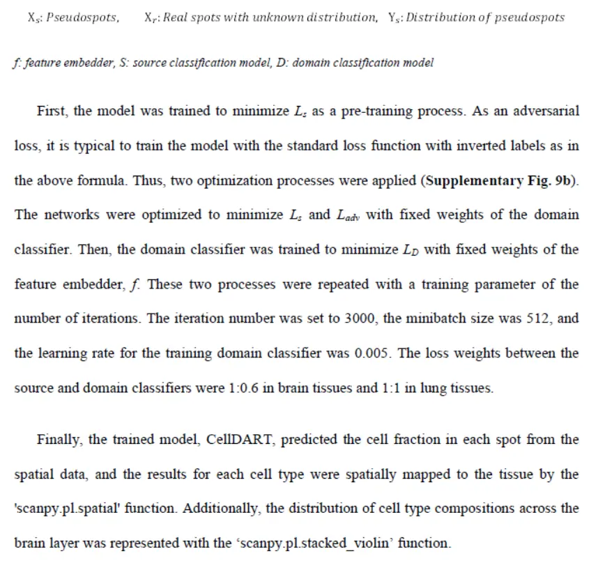
第三步 A neural network was trained to accurately decompose the pseudospots, and another network, the domain classifier, was trained to discriminate spots of real spatially resolved transcriptomes from pseudospots.（两个训练网络）

During the training process, the weights of neural networks were updated to predict cell fractions and fool the domain classifier to avoid discriminating spots and pseudospots（这个地方有点难理解，大家体会一下）。As a result, the neural network, source classifier, was trained to estimate cell fractions in both the pseudospots and the real spatial spots as an adversarial domain adaptation process（这里才算理解这个专用名称干什么的）.

到这里我们总结一下，首先用单细胞数据构建伪空间SPOT（这里用到了8个单细胞），构建的伪空间SPOT的细胞成分是知道的，然后这些伪SPOT与真实的SPOT构建神经网络，与此同时构建了细胞成分的分类器，通过一定的优化，实现真正的空间数据的细胞比例估计。

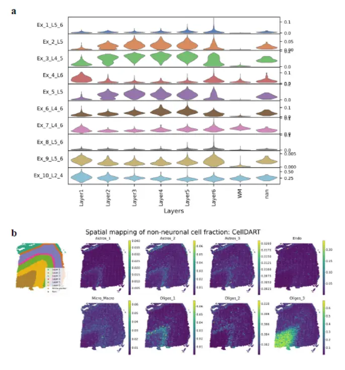
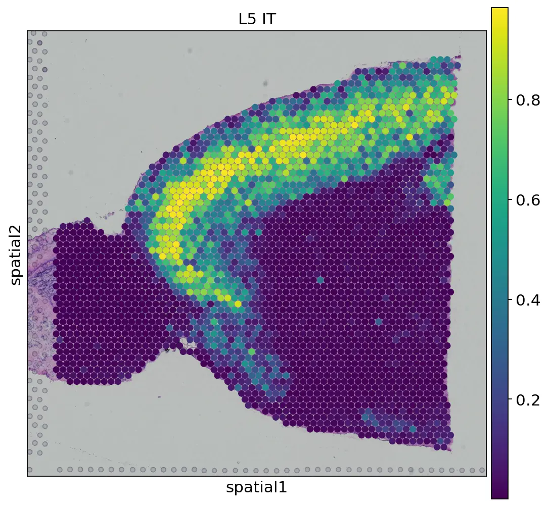
来看看解卷积效果

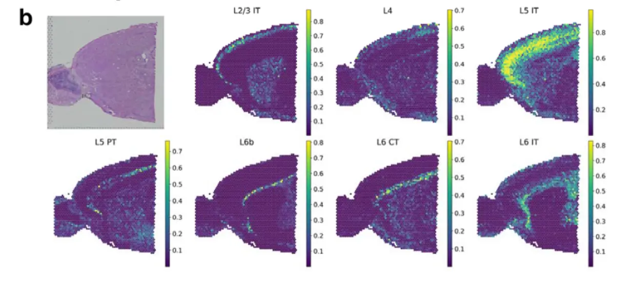
这个结果很官网的结果很相似
下面的人的数据

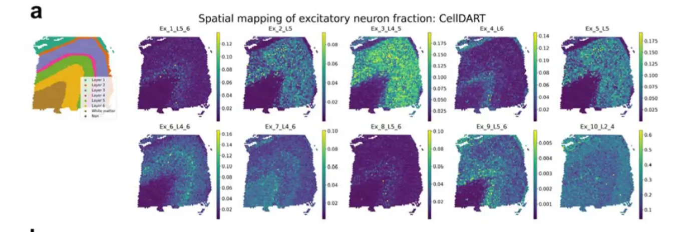
示例数据看，还可以。

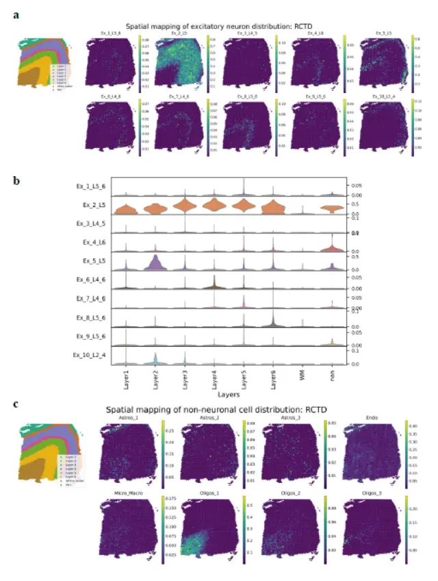
结果2 Comparison of CellDART with other integration tools in human brain tissue

• 另外三个软件是Scanorama, Cell2location, and RCTD.

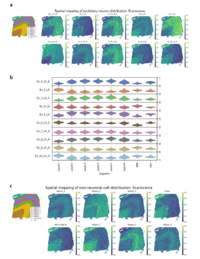
首先是Scanorama

Scanorama showed a few excitatory neurons of cortical layer-specific distribution patterns, whereas Ex_2_L5, Ex_4_L6, Ex_9_L5_6, and Ex_10_L2_4 excitatory neurons were distributed differently from the known cortical distribution（Scanorama这个方法看来不行啊）。

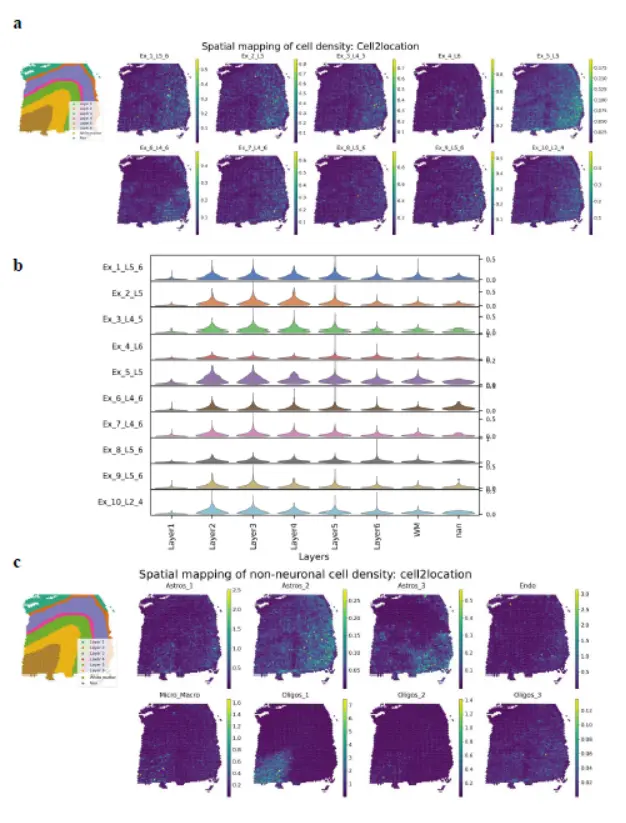
其次是Cell2location

In the case of Cell2location, neither excitatory neurons nor non-neuronal cells showed layer-specific localization patterns except for a few cell types (Ex_4_L6, Oligos_1, and Micro_Macro)（Cell2location也不行啊）

第三看RCTD

Finally, for RCTD, a few excitatory neurons (Ex_2_L5 and Ex_10_L2_4) exhibited a high cell fraction in the corresponding cortical layer of a known layer specificity; however, other excitatory neurons presented heterogeneous patterns of distribution（这更不行）

作者很贼，比较的三个软件没有一个常用的。

Receiver operating characteristic (ROC) curve analysis was implemented to compare the performance of the four different tools in predicting the layer-specific distribution of excitatory neurons

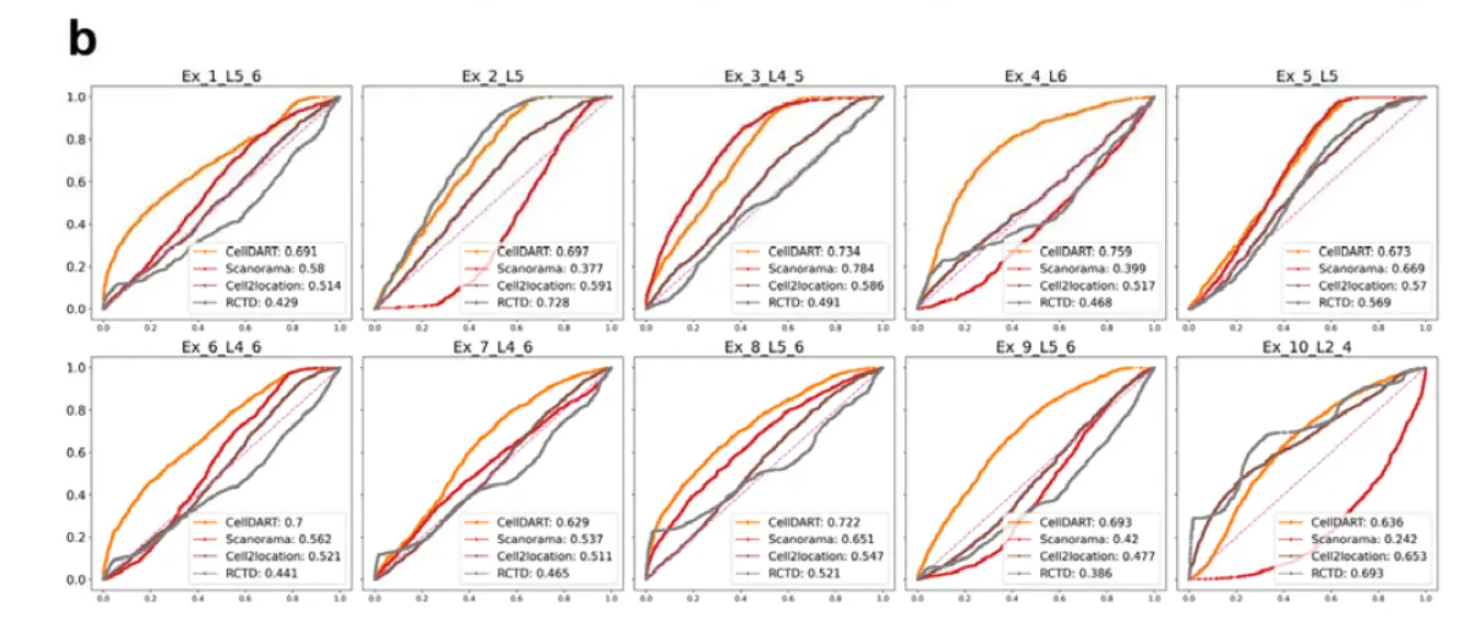
当然，文章都不用怎么看，作者的软件效果最好。

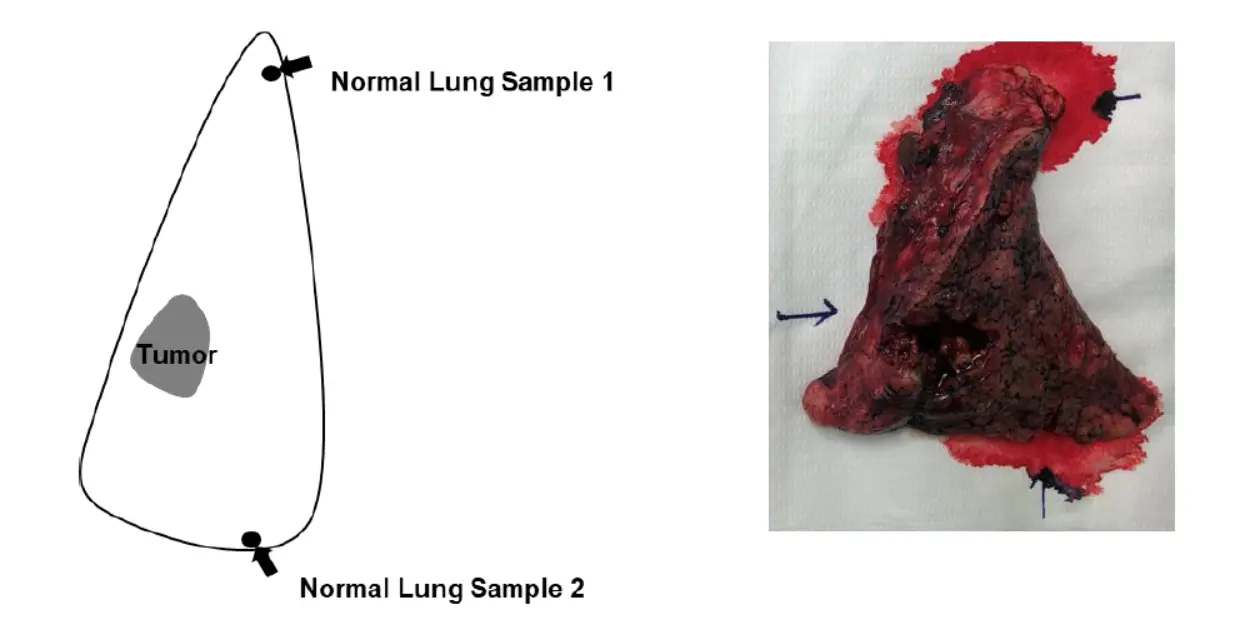
结果3 Discovery of spatial heterogeneity of human lung tissue with CellDART

CellDART was further applied to normal lung spatial transcriptomic data.（正常组织样本数据的运用）
The two normal lung tissues were dissected far from the tumor and pathologically confirmed to have no tumor cells

看看联合分析的结果

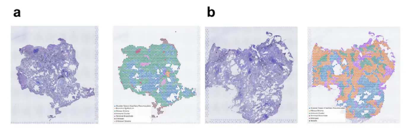
In both the lung 1 and lung 2 datasets, each cell type showed different distribution patterns across the segmented tissue domains。

 

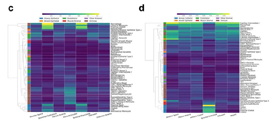
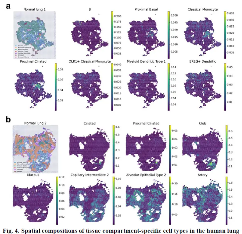
In summary, CellDART could precisely localize the spatial distribution of heterogeneous cell types in normal lung tissue.

看看文献的结论

In conclusion, CellDART is capable of estimating the spatial cell compositions in complex tissues with high levels of heterogeneity by aligning the domain of single-cell and spatial transcriptomics data. The suggested method may help elucidate the spatial interaction of various cells in close proximity and track the cell-level transcriptomic changes while preserving the spatial context.（反正就是好😄）。

Method 关注一下算法

CellDART: Cell type inference with domain adaptation

• First, a feature embedder that computes 64-dimensional embedding features from the gene expression data of either spatial spots or pseudospots was defined(首先，定义了一种特征嵌入器，该特征嵌入器根据空间点或伪点的基因表达数据计算64维嵌入特征 )。The feature embedder was comprised of two fully connected layers, each of which underwent batch normalization and activation by the ELU function（标准化和去除批次效应）。The outputs of the first layer and second layer have 1024 and 64 dimensions, respectively.（两层的维度还不一样）。
• Source and domain classifiers were defined such that they could predict the cell fraction in each spot and discriminate pseudospots from spots, respectively.（初始的分类器）。The domain classifier consisted of two fully connected layers. The first layer with 32-dimensional output was connected to the embedded features。The source classifier is directly connected to the embedded features of the feature extractor as a one-layer model connected to the feature embedder. Therefore, the feature extractor attached to either of the classifiers was named a source or domain classification model. The source and domain classification model shared the feature extractor。（理解上还是比较简单的）。

最后，看一下示例代码

CellDART Example Code: mouse brain

加载模块

import scanpy as sc
import pandas as pd
import numpy as np
import seaborn as sns
import matplotlib.pyplot as plt 
import da_cellfraction
from utils import random_mix
from sklearn.manifold import TSNE

1. Data load

load scanpy data - 10x datasets

sc.set_figure_params(facecolor="white", figsize=(8, 8))
sc.settings.verbosity = 3

adata_spatial_anterior = sc.datasets.visium_sge(
    sample_id="V1_Mouse_Brain_Sagittal_Anterior"
)
adata_spatial_posterior = sc.datasets.visium_sge(
    sample_id="V1_Mouse_Brain_Sagittal_Posterior"
)

#Normalize
for adata in [
    adata_spatial_anterior,
    adata_spatial_posterior,
]:
    sc.pp.normalize_total(adata, inplace=True)

Single cell Data: GSE115746

• Download from GEO and use two files "GSE115746_cells_exon_counts.csv" and "GSE115746_complete_metadata_28706-cells.csv"

adata_cortex = sc.read_csv('../data/GSE115746_cells_exon_counts.csv').T
adata_cortex_meta = pd.read_csv('../data/GSE115746_complete_metadata_28706-cells.csv', index_col=0)
adata_cortex_meta_ = adata_cortex_meta.loc[adata_cortex.obs.index,]
adata_cortex.obs = adata_cortex_meta_
adata_cortex.var_names_make_unique()  
#Preprocessing
adata_cortex.var['mt'] = adata_cortex.var_names.str.startswith('Mt-')  # annotate the group of mitochondrial genes as 'mt'
sc.pp.calculate_qc_metrics(adata_cortex, qc_vars=['mt'], percent_top=None, log1p=False, inplace=True)
sc.pp.normalize_total(adata_cortex)
#PCA and clustering : Known markers with 'cell_subclass'
sc.tl.pca(adata_cortex, svd_solver='arpack')
sc.pp.neighbors(adata_cortex, n_neighbors=10, n_pcs=40)
sc.tl.umap(adata_cortex)
sc.tl.leiden(adata_cortex, resolution = 0.5)
sc.pl.umap(adata_cortex, color=['leiden','cell_subclass'])

sc.tl.rank_genes_groups(adata_cortex, 'cell_subclass', method='wilcoxon')
sc.pl.rank_genes_groups(adata_cortex, n_genes=20, sharey=False)

Select same gene features

adata_spatial_anterior.var_names_make_unique() 
inter_genes = [val for val in res_genes_ if val in adata_spatial_anterior.var.index]
print('Selected Feature Gene number',len(inter_genes))
adata_cortex = adata_cortex[:,inter_genes]

adata_spatial_anterior = adata_spatial_anterior[:,inter_genes]

Array of single cell & spatial data

• Single cell data with labels
• Spatial data without labels

mat_sc = adata_cortex.X
mat_sp = adata_spatial_anterior.X.todense()

df_sc = adata_cortex.obs

lab_sc_sub = df_sc.cell_subclass
sc_sub_dict = dict(zip(range(len(set(lab_sc_sub))), set(lab_sc_sub)))
sc_sub_dict2 = dict((y,x) for x,y in sc_sub_dict.items())
lab_sc_num = [sc_sub_dict2[ii] for ii in lab_sc_sub]
lab_sc_num = np.asarray(lab_sc_num, dtype='int')

2. Generate mixture from single cell data and preprocessing

sc_mix, lab_mix = random_mix(mat_sc, lab_sc_num, nmix=5, n_samples=5000)

def log_minmaxscale(arr):
    arrd = len(arr)
    arr = np.log1p(arr)
    return (arr-np.reshape(np.min(arr,axis=1), (arrd,1)))/np.reshape((np.max(arr, axis=1)-np.min(arr,axis=1)),(arrd,1))

sc_mix_s = log_minmaxscale(sc_mix)
mat_sp_s = log_minmaxscale(mat_sp)
mat_sc_s = log_minmaxscale(mat_sc)

3. Training: Adversarial domain adaptation for cell fraction estimation

Parameters

• alpha: loss weights for adversarial learning for pooling domain classifier
• alpha_lr: learning rate for training domain classifier (alpha_lr *0.001)
• emb_dim: embedding dimension (feature dimension)
• batch_size : batch size for the training
• n_iterations: iteration number of adversarial training
• initial_train: if true, classifier model is trained firstly before adversarial domain adaptation
• initial_train_epochs: number of epochs for inital training

embs, clssmodel = da_cellfraction.train(sc_mix_s, lab_mix, mat_sp_s, 
                                 alpha=1, alpha_lr=5, emb_dim = 64, batch_size = 512,
                                 n_iterations = 2000,
                                  initial_train=True,
                                  initial_train_epochs=10)

4. Predict cell fraction of spots and visualization

pred_sp = clssmodel.predict(mat_sp_s)

def plot_cellfraction(visnum):
    adata_spatial_anterior.obs['Pred_label'] = pred_sp[:,visnum]
    sc.pl.spatial(
        adata_spatial_anterior,
        img_key="hires",
        color='Pred_label',
        palette='Set1',
        size=1.5,
        legend_loc=None,
        title = sc_sub_dict[visnum])

numlist = [2,3,7,8,12,13,18]

for num in numlist:
    plot_cellfraction(num)

方法上跟解卷积的思路一致，不过引入了新的思想，很值得一试

生活很好，有你更好