Visium HD 空间转录组分析探索之--细胞核分割

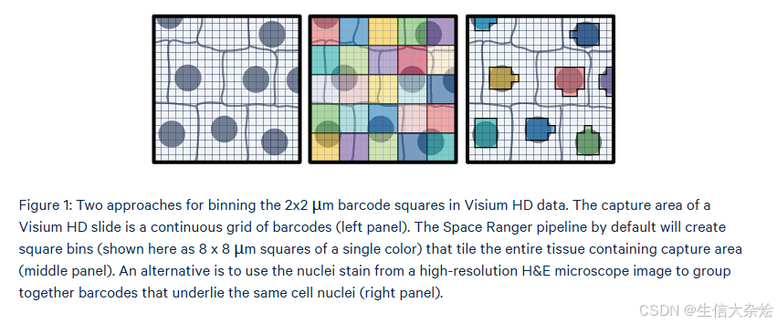
      前面我们介绍了使用单细胞数据为reference进行RCTD解卷积注释细胞类型，这种方法的好处是操作起来比较方便且结果准确，唯一一点要求就是有相应的单细胞数据，且尽可能注释详尽。10x官方也给我们提供了另一种分析方法，细胞核分割，使用高清的H&E图像识别细胞核，然后将覆盖在细胞核位置的2um bins进行合并，这样一来就得到了snRNA的结果（丢失了细胞质的基因表达信息），然后就可以下游分析了。

背景知识

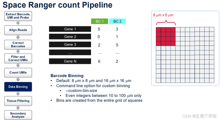
      Visium HD的捕获芯片上大概由一千一百多万个2um x 2um的小方格排列而成，切片组织覆盖在芯片捕获区上，这样2um小方格里面的探针就能去结合它上方组织的mRNA。Space Ranger会将2um小方格合并成8um x 8um或16um x 16um的bins，后续就是以这些合并后的bins为最小单元进行分析，也就是认为8um bin或这个16um bin就是一个细胞，但是这会有前面我们说的问题，细胞形状并不是规则的，并且大小也不太一样，就导致了我们认为合并后的bins它是一个细胞，其实它有可能会包含多个细胞或者只包含了细胞的一部分。

细胞核分割原理

      简单来说就是图像识别，使用高清的HE图像，基于StarDist预训练的模型，分割高分辨率的H&E图像以创建nuclei mask识别出细胞核的位置、轮廓，有了细胞核的位置信息后，就能找到有哪些2um的bin是覆盖了细胞核的，然后把这些bins合并，就完成了细胞识别。StarDist的核心是一个经过训练的神经网络模型，它能够高效地识别出图像中那些形似星星的结构。在生物医学领域，这样的形状经常出现在细胞或组织切片中，例如神经元、细胞核等。通过自动检测这些结构，StarDist极大地加速了图像分析过程，减少了人工标注的工作量。

细胞核分割优点

      根据细胞核进行bins合并，更接近单细胞数据

细胞核分割缺点

      需要有高清的HE图像，并且细胞核染色清晰，肉眼即可识别细胞核位置； 细胞核分割的方法只保留了细胞核位置的基因表达，缺失了胞质中的信息； HE图像和Cytassist图像坐标对齐的问题，即使我们已经使用loupe browser进行手动对齐，但还是会有几微米的偏差（这种偏差我们大概能知道的一个是将片子转到HD芯片上后有形变、Cytassist机器有偏差，这点10x官方也有关于固件需要升级的通知），所以我们尝试了各种数据使用细胞核分割，但是效果却仍不理想。

分析

      一定要要有高清的HE图像，并且细胞核染色清晰，肉眼即可识别细胞核位置，这个是前提。 分析代码很很简单，10x官网有详细描述https://www.10xgenomics.com/analysis-guides/segmentation-visium-hd， 同时github也有相应的封装好的代码https://github.com/10XGenomics/HumanColonCancer_VisiumHD/blob/main/Methods/NucleiSegmentation.py， 拿来就能用，要注意的是需要根据自己的数据略微调整参数

注意：下面代码是我们在10x官方给的代码基础上自己重新写的，好处是自己知道每一步干了啥，有哪些参数需要调整。总共3个函数 nuclei_segmentation() assign_bin_to_segmented_nuclei() plot_nuclei_area()

import skimage.io
from stardist import random_label_cmap
from stardist.models import StarDist2D
import matplotlib
import matplotlib.pyplot as plt
from matplotlib.colors import ListedColormap
from csbdeep.utils import normalize
from csbdeep.data import Normalizer
import numpy as np
from shapely.geometry import Polygon, Point
import anndata
# import seaborn as sns
import geopandas as gpd
import scanpy as sc
import pandas as pd
from scipy import sparse
import scipy
import gzip
def nuclei_segmentation(img, dim, block_size=4096, min_overlap=128, context=128):
  # Percentile normalization of the image
  # Adjust min_percentile and max_percentile as needed
  min_percentile = 5
  max_percentile = 95
  img = normalize(img, min_percentile, max_percentile)
  # Predict cell nuclei using the normalized image
  # Adjust nms_thresh and prob_thresh as needed
  model = StarDist2D.from_pretrained('2D_versatile_he')
  labels, polys = model.predict_instances_big(img, axes=dim, block_size=block_size,
                                            prob_thresh=0.01,nms_thresh=0.001,
                                            min_overlap=min_overlap, context=context,
                                            normalizer=None, n_tiles=(4,4,1))
  return(labels, polys)
def assign_bin_to_segmented_nuclei(gdf, adata, df_tissue_positions):
  #Set the index of the dataframe to the barcodes
  df_tissue_positions = df_tissue_positions.set_index('barcode')
  # Create an index in the dataframe to check joins
  df_tissue_positions['index']=df_tissue_positions.index
  print("... Creating bin coordinate GeoDataFrame ...")
  # Create a GeoDataFrame for bin coordinates
  geometry = [Point(xy) for xy in zip(df_tissue_positions['pxl_col_in_fullres'],
                                    df_tissue_positions['pxl_row_in_fullres'])]
  gdf_coordinates = gpd.GeoDataFrame(df_tissue_positions, geometry=geometry)
  print("... Overlapping bins with nuclei ...")
  # Perform a spatial join to check which coordinates are in a polygon
  result_spatial_join = gpd.sjoin(gdf_coordinates, gdf,
                                how='left', predicate='within')
  print("... Filtering bins ...")
  # Identify the bins that are in a nuclues and find bins that are in more than one nuclues
  result_spatial_join['is_within_polygon'] = ~result_spatial_join['index_right'].isna()
  barcodes_in_overlaping_polygons = pd.unique(result_spatial_join[result_spatial_join.duplicated(subset=['index'])]['index'])
  result_spatial_join['is_not_in_an_polygon_overlap'] = ~result_spatial_join['index'].isin(barcodes_in_overlaping_polygons)
  # Remove barcodes in overlapping nuclei
  barcodes_in_one_polygon = result_spatial_join[result_spatial_join['is_within_polygon'] &
                                              result_spatial_join['is_not_in_an_polygon_overlap']]
  # The AnnData object is filtered to only contain the barcodes that are in non-overlapping polygon regions
  filtered_obs_mask = adata.obs_names.isin(barcodes_in_one_polygon['index'])
  filtered_adata = adata[filtered_obs_mask,:]
  print("... Counting gene expression from overlapped bins for each nucleus ...")
  # Add the results of the point spatial join to the Anndata object
  filtered_adata.obs =  pd.merge(filtered_adata.obs,
                                 barcodes_in_one_polygon[['index','geometry','id',
                                                        'is_within_polygon',
                                                        'is_not_in_an_polygon_overlap']],
                                 left_index=True, right_index=True)
  # Group the data by unique nucleous IDs
  groupby_object = filtered_adata.obs.groupby(['id'], observed=True)
  # Extract the gene expression counts from the AnnData object
  counts = filtered_adata.X
  # Obtain the number of unique nuclei and the number of genes in the expression data
  N_groups = groupby_object.ngroups
  N_genes = counts.shape[1]
  # Initialize a sparse matrix to store the summed gene counts for each nucleus
  summed_counts = sparse.lil_matrix((N_groups, N_genes))
  # Lists to store the IDs of polygons and the current row index
  polygon_id = []
  row = 0
  # Iterate over each unique polygon to calculate the sum of gene counts.
  for polygons, idx_ in groupby_object.indices.items():
      summed_counts[row] = counts[idx_].sum(0)
      row += 1
      polygon_id.append(polygons)
  # Create and AnnData object from the summed count matrix
  summed_counts = summed_counts.tocsr()
  grouped_filtered_adata = anndata.AnnData(X=summed_counts,
                                           obs=pd.DataFrame(polygon_id,
                                                            columns=['id'],
                                                            index=polygon_id),
                                           var=filtered_adata.var)
  return(grouped_filtered_adata)
def plot_nuclei_area(gdf,area_cut_off):
    fig, axs = plt.subplots(1, 2, figsize=(15, 4))
    # Plot the histograms
    axs[0].hist(gdf['area'], bins=50, edgecolor='black')
    axs[0].set_title('Nuclei Area')
    axs[1].hist(gdf[gdf['area'] < area_cut_off]['area'], bins=50, edgecolor='black')
    axs[1].set_title('Nuclei Area Filtered:'+str(area_cut_off))
    plt.tight_layout()
    plt.show()

step1. 开始细胞核分割

plt.figure(figsize=(8,6))
plt.imshow(img,cmap='gray')
img = skimage.io.imread('./CRC/P1_CRC/images', plugin='tifffile')
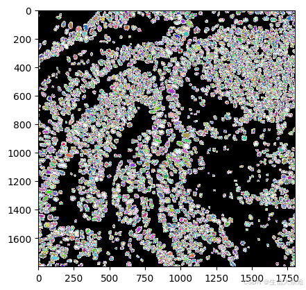
labels, polys = nuclei_segmentation(img, "YXC", block_size=512, min_overlap=64, context=96)
lbl_cmap = random_label_cmap()
plt.imshow(labels,cmap=lbl_cmap)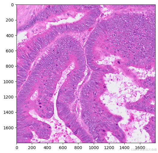

 step2. Convert segmentation results into Geodataframe for barcode binning

# Convert polys to geometries
geometries = []
# Iterate over each nuclei detected in the image
for nuclei in range(len(polys['coord'])):
    # Extract the x and y coordinates
    coords = [(y, x) for x, y in zip(polys['coord'][nuclei][0], polys['coord'][nuclei][1])]
    # Add the polygon to the list of geometries
    geometries.append(Polygon(coords))
# Create the geodataframe
gdf = gpd.GeoDataFrame(geometry=geometries)
# Add a unique ID column
gdf['id'] = [f"ID_{i+1}" for i, _ in enumerate(gdf.index)]
gdf.head()
x_min = 1000
x_max = 1512
y_min = 400
y_max = 984
bbox = (x_min,y_min,x_max,y_max)
cropped_img = img[bbox[1]:bbox[3], bbox[0]:bbox[2],:]
 # Plot options
fig, axes = plt.subplots(1, 2, figsize=(12, 6))
# Plot the cropped image
axes[0].imshow(cropped_img, cmap='gray', origin='lower')
axes[0].axis('off')
trim = 10
bbox_polygon = Polygon([(bbox[0]+trim, bbox[1]+trim),
                         (bbox[2]-trim, bbox[1]+trim),
                          (bbox[2]-trim, bbox[3]-trim),
                           (bbox[0]+trim, bbox[3]-trim)])
# Filter for polygons in the box
intersects_bbox = gdf['geometry'].intersects(bbox_polygon)
filtered_gdf = gdf[intersects_bbox]
filtered_gdf.plot(cmap=ListedColormap(['grey']), ax=axes[1])
axes[1].axis('off')
plt.show()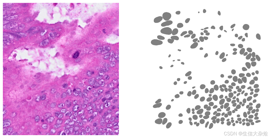

step3. Assign 2x2 micron bins to nuclei

# Read Visium HD data 2x2 micron bin feature barcode count matrix in h5
adata = sc.read_10x_h5("./2micron_filtered_feature_bc_matrix_demo.h5")
# read the spatial coordinates of 2x2 micron bin
df_tissue_positions = pd.read_parquet("./2micron_tissue_positions_demo.parquet")
grouped_filtered_adata = assign_bin_to_segmented_nuclei(gdf, adata, df_tissue_positions)

step4. Filter nuclei

      我们使用stardist进行细胞核识别，但是有的时候识别的不是很准确，比如某些细胞离得很近，或者细胞之间有覆盖，从图像上看这几个细胞核离的很近，然后这几个核可能就被识别成一个核了，所以我们要根据识别出来核的大小进行过滤。

gdf['area'] = gdf['geometry'].area
plot_nuclei_area(gdf=gdf,area_cut_off=1000)
# Calculate quality control metrics for the original AnnData object
sc.pp.calculate_qc_metrics(grouped_filtered_adata, percent_top=None, inplace=True)
# Create a mask based on the 'id' column for values present in 'gdf' with 'area' less than 1000
mask_area = grouped_filtered_adata.obs['id'].isin(gdf[gdf['area'] < 1000].id)
# Create a mask based on the 'total_counts' column for values greater than 50
mask_count = grouped_filtered_adata.obs['total_counts'] > 50
# Apply both masks to the original AnnData to create a new filtered AnnData object
count_area_filtered_adata = grouped_filtered_adata[mask_area & mask_count, :]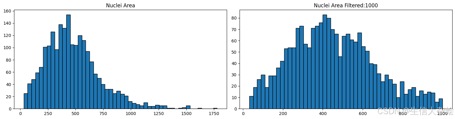

 讨论

      通过观察与组织形态学相匹配的标记表达和聚类来验证结果。这种方法对于具有清晰定义的大细胞核且易于区分彼此和背景的图像最为有效。对于任何新的H&E切片和Visium HD 基因表达数据集，可能都需要对参数进行优化。需要牢记的关键参数是概率阈值、聚类分辨率以及总 UMI和细胞核大小过滤器截止值。

      除了参数优化外，该方法还有一些改进可以提高结果。在示例使用了StarDist的预训练H&E分类器模型。这超出了本分析指南的范围，但 starDist 可以使用自定义训练模型。此外，示例只考虑了核信息。在核mask中扩展每个单独核的边界可以提高结果。

微信公众号：生信大杂烩