基于多层感知器的姓氏分类

使用多层感知器进行姓氏分类

1. 实验内容

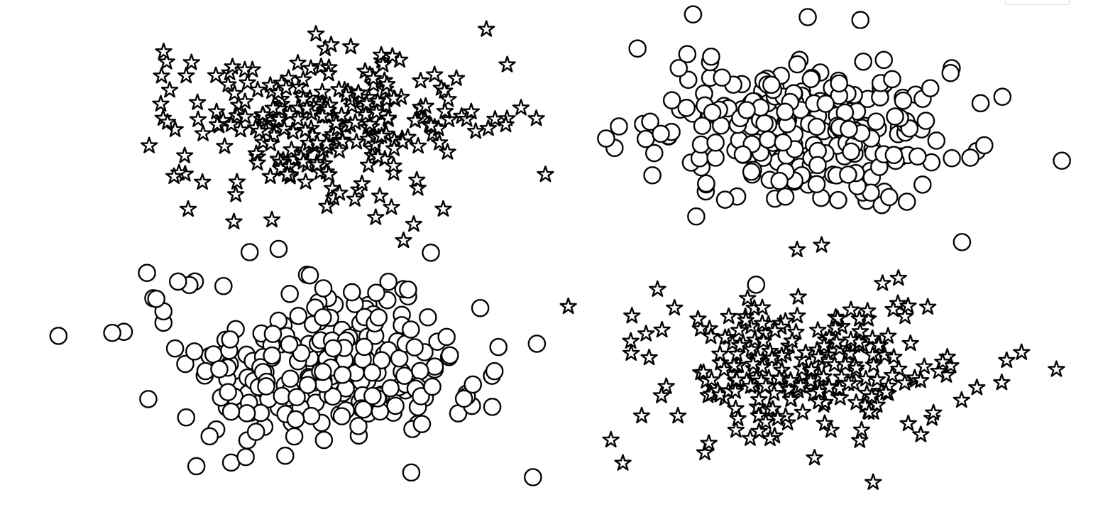
在实验3中，我们通过观察感知器来介绍神经网络的基础，感知器是现存最简单的神经网络。感知器的一个历史性的缺点是它不能学习数据中存在的一些非常重要的模式。例如，查看图4-1中绘制的数据点。这相当于非此即彼(XOR)的情况，在这种情况下，决策边界不能是一条直线(也称为线性可分)。在这个例子中，感知器失败了。

图4-1 XOR数据集中的两个类绘制为圆形和星形。请注意，没有任何一行可以分隔这两个类。

在这一实验中，我们将探索传统上称为前馈网络的神经网络模型，以及两种前馈神经网络:多层感知器和卷积神经网络。多层感知器在结构上扩展了我们在实验3中研究的简单感知器，将多个感知器分组在一个单层，并将多个层叠加在一起。我们稍后将介绍多层感知器，并在“示例:带有多层感知器的姓氏分类”中展示它们在多层分类中的应用。

本实验研究的第二种前馈神经网络，卷积神经网络，在处理数字信号时深受窗口滤波器的启发。通过这种窗口特性，卷积神经网络能够在输入中学习局部化模式，这不仅使其成为计算机视觉的主轴，而且是检测单词和句子等序列数据中的子结构的理想候选。我们在“卷积神经网络”中概述了卷积神经网络，并在“示例:使用CNN对姓氏进行分类”中演示了它们的使用。

在本实验中，多层感知器和卷积神经网络被分组在一起，因为它们都是前馈神经网络，并且与另一类神经网络——递归神经网络(RNNs)形成对比，递归神经网络(RNNs)允许反馈(或循环)，这样每次计算都可以从之前的计算中获得信息。在实验6和实验7中，我们将介绍RNNs以及为什么允许网络结构中的循环是有益的。

在我们介绍这些不同的模型时，需要理解事物如何工作的一个有用方法是在计算数据张量时注意它们的大小和形状。每种类型的神经网络层对它所计算的数据张量的大小和形状都有特定的影响，理解这种影响可以极大地有助于对这些模型的深入理解。

2. 实验要点

• 通过“示例:带有多层感知器的姓氏分类”，掌握多层感知器在多层分类中的应用
• 掌握每种类型的神经网络层对它所计算的数据张量的大小和形状的影响

3. 实验环境

• Python 3.6.7

二、The Multilayer Perceptron（多层感知器）

多层感知器(MLP)被认为是最基本的神经网络构建模块之一。最简单的MLP是对第3章感知器的扩展。感知器将数据向量作为输入，计算出一个输出值。在MLP中，许多感知器被分组，以便单个层的输出是一个新的向量，而不是单个输出值。在PyTorch中，正如您稍后将看到的，这只需设置线性层中的输出特性的数量即可完成。MLP的另一个方面是，它将多个层与每个层之间的非线性结合在一起。

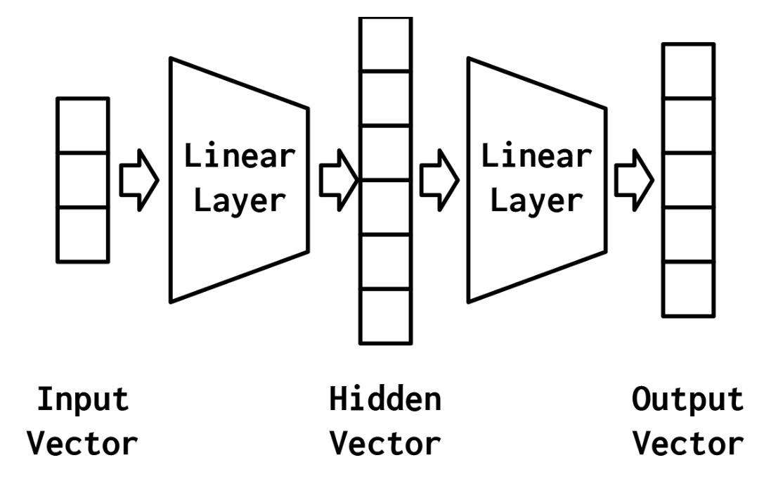
最简单的MLP，如图4-2所示，由三个表示阶段和两个线性层组成。第一阶段是输入向量。这是给定给模型的向量。在“示例:对餐馆评论的情绪进行分类”中，输入向量是Yelp评论的一个收缩的one-hot表示。给定输入向量，第一个线性层计算一个隐藏向量——表示的第二阶段。隐藏向量之所以这样被调用，是因为它是位于输入和输出之间的层的输出。我们所说的“层的输出”是什么意思?理解这个的一种方法是隐藏向量中的值是组成该层的不同感知器的输出。使用这个隐藏的向量，第二个线性层计算一个输出向量。在像Yelp评论分类这样的二进制任务中，输出向量仍然可以是1。在多类设置中，将在本实验后面的“示例:带有多层感知器的姓氏分类”一节中看到，输出向量是类数量的大小。虽然在这个例子中，我们只展示了一个隐藏的向量，但是有可能有多个中间阶段，每个阶段产生自己的隐藏向量。最终的隐藏向量总是通过线性层和非线性的组合映射到输出向量。

图4-2 一种具有两个线性层和三个表示阶段（输入向量、隐藏向量和输出向量)的MLP的可视化表示

mlp的力量来自于添加第二个线性层和允许模型学习一个线性分割的的中间表示——该属性的能表示一个直线(或更一般的,一个超平面)可以用来区分数据点落在线(或超平面)的哪一边的。学习具有特定属性的中间表示，如分类任务是线性可分的，这是使用神经网络的最深刻后果之一，也是其建模能力的精髓。在下一节中，我们将更深入地研究这意味着什么。

2.1 A Simple Example: XOR

让我们看一下前面描述的XOR示例，看看感知器与MLP之间会发生什么。在这个例子中，我们在一个二元分类任务中训练感知器和MLP:星和圆。每个数据点是一个二维坐标。在不深入研究实现细节的情况下，最终的模型预测如图4-3所示。在这个图中，错误分类的数据点用黑色填充，而正确分类的数据点没有填充。在左边的面板中，从填充的形状可以看出，感知器在学习一个可以将星星和圆分开的决策边界方面有困难。然而，MLP(右面板)学习了一个更精确地对恒星和圆进行分类的决策边界。

图4-3 从感知器(左)和MLP(右)学习的XOR问题的解决方案显示

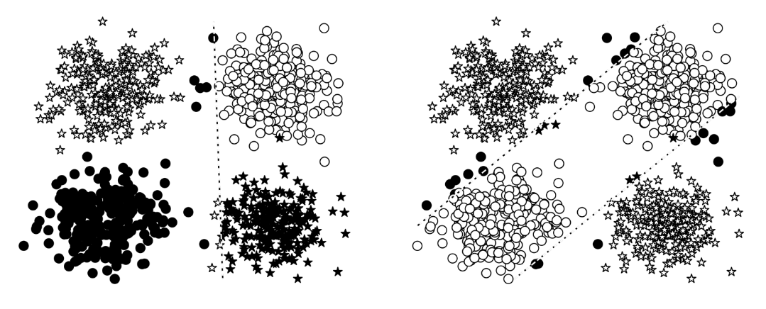
图4-3中，每个数据点的真正类是该点的形状:星形或圆形。错误的分类用块填充，正确的分类没有填充。这些线是每个模型的决策边界。在边的面板中，感知器学习—个不能正确地将圆与星分开的决策边界。事实上，没有一条线可以。在右动的面板中，MLP学会了从圆中分离星。

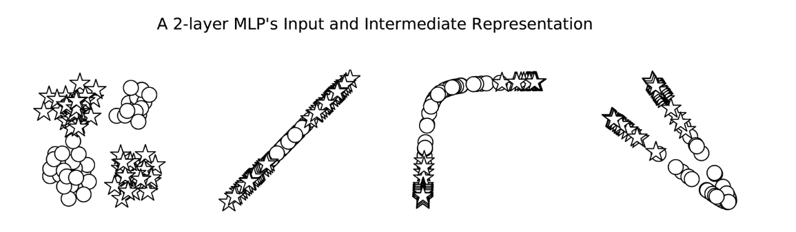
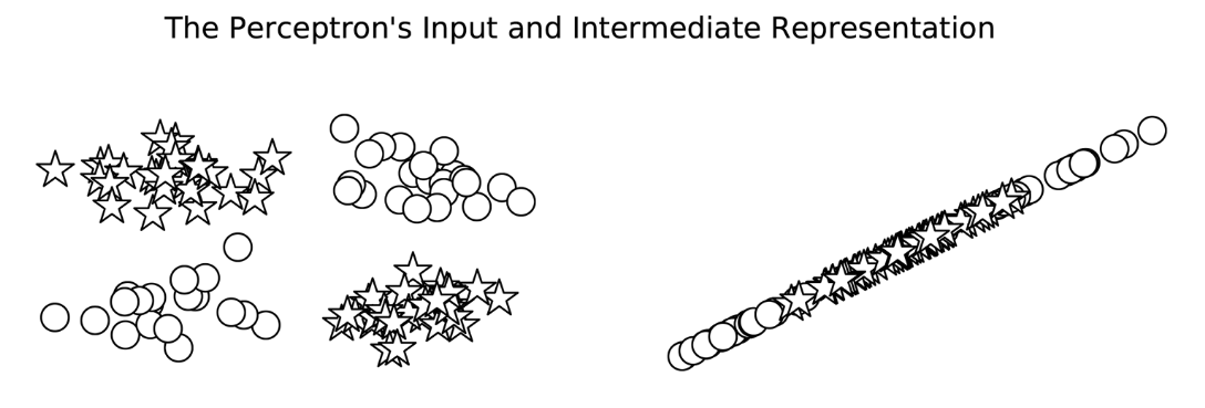
虽然在图中显示MLP有两个决策边界，这是它的优点，但它实际上只是一个决策边界!决策边界就是这样出现的，因为中间表示法改变了空间，使一个超平面同时出现在这两个位置上。在图4-4中，我们可以看到MLP计算的中间值。这些点的形状表示类(星形或圆形)。我们所看到的是，神经网络(本例中为MLP)已经学会了“扭曲”数据所处的空间，以便在数据通过最后一层时，用一线来分割它们。

图4-4 MLP的输入和中间表示是可视化的。从左到右:（1）网络的输入;（2）第一个线性模块的输出;（3）第一个非线性模块的输出;（4）第二个线性模块的输出。第一个线性模块的输出将圆和星分组，而第二个线性模块的输出将数据点重新组织为线性可分的。

相反，如图4-5所示，感知器没有额外的一层来处理数据的形状，直到数据变成线性可分的。

图4-5 感知器的输入和输出表示。因为它没有像MLP那样的中间表示来分组和重新组织，所以它不能将圆和星分开。

2.2 Implementing MLPs in PyTorch

在上一节中，我们概述了MLP的核心思想。在本节中，我们将介绍PyTorch中的一个实现。如前所述，MLP除了实验3中简单的感知器之外，还有一个额外的计算层。在我们在例4-1中给出的实现中，我们用PyTorch的两个线性模块实例化了这个想法。线性对象被命名为fc1和fc2，它们遵循一个通用约定，即将线性模块称为“完全连接层”，简称为“fc层”。除了这两个线性层外，还有一个修正的线性单元(ReLU)非线性(在实验3“激活函数”一节中介绍)，它在被输入到第二个线性层之前应用于第一个线性层的输出。由于层的顺序性，必须确保层中的输出数量等于下一层的输入数量。使用两个线性层之间的非线性是必要的，因为没有它，两个线性层在数学上等价于一个线性层4，因此不能建模复杂的模式。MLP的实现只实现反向传播的前向传递。这是因为PyTorch根据模型的定义和向前传递的实现，自动计算出如何进行向后传递和梯度更新。

Example 4-1. Multilayer Perceptron

from collections import Counter
import json
import os
import string

import numpy as np
import pandas as pd

import torch
import torch.nn as nn
import torch.nn.functional as F
import torch.optim as optim
from torch.utils.data import Dataset, DataLoader
from tqdm import tqdm_notebook

class MultilayerPerceptron(nn.Module):
    def __init__(self, input_dim, hidden_dim, output_dim):
        """
        Args:
            input_dim (int): the size of the input vectors
            hidden_dim (int): the output size of the first Linear layer
            output_dim (int): the output size of the second Linear layer
        """
        super(MultilayerPerceptron, self).__init__()
        self.fc1 = nn.Linear(input_dim, hidden_dim)
        self.fc2 = nn.Linear(hidden_dim, output_dim)

    def forward(self, x_in, apply_softmax=False):
        """The forward pass of the MLP

        Args:
            x_in (torch.Tensor): an input data tensor.
                x_in.shape should be (batch, input_dim)
            apply_softmax (bool): a flag for the softmax activation
                should be false if used with the Cross Entropy losses
        Returns:
            the resulting tensor. tensor.shape should be (batch, output_dim)
        """
        intermediate = F.relu(self.fc1(x_in))
        output = self.fc2(intermediate)

        if apply_softmax:
            output = F.softmax(output, dim=1)
        return output

在例4-2中，我们实例化了MLP。由于MLP实现的通用性，可以为任何大小的输入建模。为了演示，我们使用大小为3的输入维度、大小为4的输出维度和大小为100的隐藏维度。请注意，在print语句的输出中，每个层中的单元数很好地排列在一起，以便为维度3的输入生成维度4的输出。

Example 4-2. An example instantiation of an MLP

input_dim = 3
hidden_dim = 100
output_dim = 4

# Initialize model
mlp = MultilayerPerceptron(input_dim, hidden_dim, output_dim)
print(mlp)

我们可以通过传递一些随机输入来快速测试模型的“连接”，如示例4-3所示。因为模型还没有经过训练，所以输出是随机的。在花费时间训练模型之前，这样做是一个有用的完整性检查。请注意PyTorch的交互性是如何让我们在开发过程中实时完成所有这些工作的，这与使用NumPy或panda没有太大区别:

Example 4-3. Testing the MLP with random inputs

def describe(x):
    print("Type: {}".format(x.type()))
    print("Shape/size: {}".format(x.shape))
    print("Values: \n{}".format(x))

x_input = torch.rand(batch_size, input_dim)
describe(x_input)

上述代码运行结果：

Type: torch.FloatTensor
Shape/size: torch.Size([2, 3])
Values: 
tensor([[0.6193, 0.7045, 0.7812],
        [0.6345, 0.4476, 0.9909]])

y_output = mlp(x_input, apply_softmax=False)
describe(y_output)

上述代码运行结果：

Type: torch.FloatTensor
Shape/size: torch.Size([2, 4])
Values: 
tensor([[ 0.2356,  0.0983, -0.0111, -0.0156],
        [ 0.1604,  0.1586, -0.0642,  0.0010]], grad_fn=<AddmmBackward>)

学习如何读取PyTorch模型的输入和输出非常重要。在前面的例子中，MLP模型的输出是一个有两行四列的张量。这个张量中的行与批处理维数对应，批处理维数是小批处理中的数据点的数量。列是每个数据点的最终特征向量。在某些情况下，例如在分类设置中，特征向量是一个预测向量。名称为“预测向量”表示它对应于一个概率分布。预测向量会发生什么取决于我们当前是在进行训练还是在执行推理。在训练期间，输出按原样使用，带有一个损失函数和目标类标签的表示。我们将在“示例:带有多层感知器的姓氏分类”中对此进行深入介绍。

但是，如果想将预测向量转换为概率，则需要额外的步骤。具体来说，需要softmax函数，它用于将一个值向量转换为概率。softmax有许多根。在物理学中，它被称为玻尔兹曼或吉布斯分布;在统计学中，它是多项式逻辑回归;在自然语言处理(NLP)社区，它是最大熵(MaxEnt)分类器。不管叫什么名字，这个函数背后的直觉是，大的正值会导致更高的概率，小的负值会导致更小的概率。在示例4-3中，apply_softmax参数应用了这个额外的步骤。在例4-4中，可以看到相同的输出，但是这次将apply_softmax标志设置为True:

Example 4-4. MLP with apply_softmax=True

y_output = mlp(x_input, apply_softmax=True)
describe(y_output)

上述代码运行结果：

Type: torch.FloatTensor
Shape/size: torch.Size([2, 4])
Values: 
tensor([[0.2915, 0.2541, 0.2277, 0.2267],
        [0.2740, 0.2735, 0.2189, 0.2336]], grad_fn=<SoftmaxBackward>)

综上所述，mlp是将张量映射到其他张量的线性层。在每一对线性层之间使用非线性来打破线性关系，并允许模型扭曲向量空间。在分类设置中，这种扭曲应该导致类之间的线性可分性。另外，可以使用softmax函数将MLP输出解释为概率，但是不应该将softmax与特定的损失函数一起使用，因为底层实现可以利用高级数学/计算捷径。

三、实验步骤

3.1 Example: Surname Classification with a Multilayer Perceptron

在本节中，我们将MLP应用于将姓氏分类到其原籍国的任务。从公开观察到的数据推断人口统计信息(如国籍)具有从产品推荐到确保不同人口统计用户获得公平结果的应用。人口统计和其他自我识别信息统称为“受保护属性”。“在建模和产品中使用这些属性时，必须小心。”我们首先对每个姓氏的字符进行拆分，并像对待“示例:将餐馆评论的情绪分类”中的单词一样对待它们。除了数据上的差异，字符层模型在结构和实现上与基于单词的模型基本相似.

应该从这个例子中吸取的一个重要教训是，MLP的实现和训练是从我们在第3章中看到的感知器的实现和培训直接发展而来的。事实上，我们在实验3中提到了这个例子，以便更全面地了解这些组件。此外，我们不包括“例子:餐馆评论的情绪分类”中看到的代码。

本节的其余部分将从姓氏数据集及其预处理步骤的描述开始。然后，我们使用词汇表、向量化器和DataLoader类逐步完成从姓氏字符串到向量化小批处理的管道。如果你通读了实验3，应该知道，这里只是做了一些小小的修改。

我们将通过描述姓氏分类器模型及其设计背后的思想过程来继续本节。MLP类似于我们在实验3中看到的感知器例子，但是除了模型的改变，我们在这个例子中引入了多类输出及其对应的损失函数。在描述了模型之后，我们完成了训练例程。训练程序与“示例:对餐馆评论的情绪进行分类”非常相似，因此为了简洁起见，我们在这里不像在该部分中那样深入，可以回顾这一节内容。

3.1.1 The Surname Dataset

姓氏数据集，它收集了来自18个不同国家的10,000个姓氏，这些姓氏是作者从互联网上不同的姓名来源收集的。该数据集将在本课程实验的几个示例中重用，并具有一些使其有趣的属性。第一个性质是它是相当不平衡的。排名前三的课程占数据的60%以上:27%是英语，21%是俄语，14%是阿拉伯语。剩下的15个民族的频率也在下降——这也是语言特有的特性。第二个特点是，在国籍和姓氏正字法(拼写)之间有一种有效和直观的关系。有些拼写变体与原籍国联系非常紧密(比如“O ‘Neill”、“Antonopoulos”、“Nagasawa”或“Zhu”)。

为了创建最终的数据集，我们从一个比课程补充材料中包含的版本处理更少的版本开始，并执行了几个数据集修改操作。第一个目的是减少这种不平衡——原始数据集中70%以上是俄文，这可能是由于抽样偏差或俄文姓氏的增多。为此，我们通过选择标记为俄语的姓氏的随机子集对这个过度代表的类进行子样本。接下来，我们根据国籍对数据集进行分组，并将数据集分为三个部分:70%到训练数据集，15%到验证数据集，最后15%到测试数据集，以便跨这些部分的类标签分布具有可比性。

SurnameDataset的实现与“Example: classification of Sentiment of Restaurant Reviews”中的ReviewDataset几乎相同，只是在getitem方法的实现方式上略有不同。回想一下，本课程中呈现的数据集类继承自PyTorch的数据集类，因此，我们需要实现两个函数:__getitem方法，它在给定索引时返回一个数据点;以及len方法，该方法返回数据集的长度。“示例:餐厅评论的情绪分类”中的示例与本示例的区别在getitem__中，如示例4-5所示。它不像“示例:将餐馆评论的情绪分类”那样返回一个向量化的评论，而是返回一个向量化的姓氏和与其国籍相对应的索引:

Example 4-5. Implementing SurnameDataset.__getitem__()

class SurnameDataset(Dataset):
    def __init__(self, surname_df, vectorizer):
        """
        Args:
            surname_df (pandas.DataFrame): the dataset
            vectorizer (SurnameVectorizer): vectorizer instatiated from dataset
        """
        self.surname_df = surname_df
        self._vectorizer = vectorizer

        self.train_df = self.surname_df[self.surname_df.split=='train']
        self.train_size = len(self.train_df)

        self.val_df = self.surname_df[self.surname_df.split=='val']
        self.validation_size = len(self.val_df)

        self.test_df = self.surname_df[self.surname_df.split=='test']
        self.test_size = len(self.test_df)

        self._lookup_dict = {'train': (self.train_df, self.train_size),
                             'val': (self.val_df, self.validation_size),
                             'test': (self.test_df, self.test_size)}

        self.set_split('train')
        
        # Class weights
        class_counts = surname_df.nationality.value_counts().to_dict()
        def sort_key(item):
            return self._vectorizer.nationality_vocab.lookup_token(item[0])
        sorted_counts = sorted(class_counts.items(), key=sort_key)
        frequencies = [count for _, count in sorted_counts]
        self.class_weights = 1.0 / torch.tensor(frequencies, dtype=torch.float32)

    @classmethod
    def load_dataset_and_make_vectorizer(cls, surname_csv):
        """Load dataset and make a new vectorizer from scratch
        
        Args:
            surname_csv (str): location of the dataset
        Returns:
            an instance of SurnameDataset
        """
        surname_df = pd.read_csv(surname_csv)
        train_surname_df = surname_df[surname_df.split=='train']
        return cls(surname_df, SurnameVectorizer.from_dataframe(train_surname_df))

    @classmethod
    def load_dataset_and_load_vectorizer(cls, surname_csv, vectorizer_filepath):
        """Load dataset and the corresponding vectorizer. 
        Used in the case in the vectorizer has been cached for re-use
        
        Args:
            surname_csv (str): location of the dataset
            vectorizer_filepath (str): location of the saved vectorizer
        Returns:
            an instance of SurnameDataset
        """
        surname_df = pd.read_csv(surname_csv)
        vectorizer = cls.load_vectorizer_only(vectorizer_filepath)
        return cls(surname_df, vectorizer)

    @staticmethod
    def load_vectorizer_only(vectorizer_filepath):
        """a static method for loading the vectorizer from file
        
        Args:
            vectorizer_filepath (str): the location of the serialized vectorizer
        Returns:
            an instance of SurnameVectorizer
        """
        with open(vectorizer_filepath) as fp:
            return SurnameVectorizer.from_serializable(json.load(fp))

    def save_vectorizer(self, vectorizer_filepath):
        """saves the vectorizer to disk using json
        
        Args:
            vectorizer_filepath (str): the location to save the vectorizer
        """
        with open(vectorizer_filepath, "w") as fp:
            json.dump(self._vectorizer.to_serializable(), fp)

    def get_vectorizer(self):
        """ returns the vectorizer """
        return self._vectorizer

    def set_split(self, split="train"):
        """ selects the splits in the dataset using a column in the dataframe """
        self._target_split = split
        self._target_df, self._target_size = self._lookup_dict[split]

    def __len__(self):
        return self._target_size

    def __getitem__(self, index):
        """the primary entry point method for PyTorch datasets
        
        Args:
            index (int): the index to the data point 
        Returns:
            a dictionary holding the data point's:
                features (x_surname)
                label (y_nationality)
        """
        row = self._target_df.iloc[index]

        surname_vector = \
            self._vectorizer.vectorize(row.surname)

        nationality_index = \
            self._vectorizer.nationality_vocab.lookup_token(row.nationality)

        return {'x_surname': surname_vector,
                'y_nationality': nationality_index}

    def get_num_batches(self, batch_size):
        """Given a batch size, return the number of batches in the dataset
        
        Args:
            batch_size (int)
        Returns:
            number of batches in the dataset
        """
        return len(self) // batch_size

    
def generate_batches(dataset, batch_size, shuffle=True,
                     drop_last=True, device="cpu"): 
    """
    A generator function which wraps the PyTorch DataLoader. It will 
      ensure each tensor is on the write device location.
    """
    dataloader = DataLoader(dataset=dataset, batch_size=batch_size,
                            shuffle=shuffle, drop_last=drop_last)

    for data_dict in dataloader:
        out_data_dict = {}
        for name, tensor in data_dict.items():
            out_data_dict[name] = data_dict[name].to(device)
        yield out_data_dict

3.1.2 Vocabulary, Vectorizer, and DataLoader

为了使用字符对姓氏进行分类，我们使用词汇表、向量化器和DataLoader将姓氏字符串转换为向量化的minibatches。这些数据结构与“Example: Classifying Sentiment of Restaurant Reviews”中使用的数据结构相同，它们举例说明了一种多态性，这种多态性将姓氏的字符标记与Yelp评论的单词标记相同对待。数据不是通过将字令牌映射到整数来向量化的，而是通过将字符映射到整数来向量化的。

THE VOCABULARY CLASS

本例中使用的词汇类与“example: Classifying Sentiment of Restaurant Reviews”中的词汇完全相同，该词汇类将Yelp评论中的单词映射到对应的整数。简要概述一下，词汇表是两个Python字典的协调，这两个字典在令牌(在本例中是字符)和整数之间形成一个双射;也就是说，第一个字典将字符映射到整数索引，第二个字典将整数索引映射到字符。add_token方法用于向词汇表中添加新的令牌，lookup_token方法用于检索索引，lookup_index方法用于检索给定索引的令牌(在推断阶段很有用)。与Yelp评论的词汇表不同，我们使用的是one-hot词汇表，不计算字符出现的频率，只对频繁出现的条目进行限制。这主要是因为数据集很小，而且大多数字符足够频繁。

THE SURNAMEVECTORIZER

虽然词汇表将单个令牌(字符)转换为整数，但SurnameVectorizer负责应用词汇表并将姓氏转换为向量。实例化和使用非常类似于“示例:对餐馆评论的情绪进行分类”中的ReviewVectorizer，但有一个关键区别:字符串没有在空格上分割。姓氏是字符的序列，每个字符在我们的词汇表中是一个单独的标记。然而，在“卷积神经网络”出现之前，我们将忽略序列信息，通过迭代字符串输入中的每个字符来创建输入的收缩one-hot向量表示。我们为以前未遇到的字符指定一个特殊的令牌，即UNK。由于我们仅从训练数据实例化词汇表，而且验证或测试数据中可能有惟一的字符，所以在字符词汇表中仍然使用UNK符号。

虽然我们在这个示例中使用了收缩的one-hot，但是在后面的实验中，将了解其他向量化方法，它们是one-hot编码的替代方法，有时甚至更好。具体来说，在“示例:使用CNN对姓氏进行分类”中，将看到一个热门矩阵，其中每个字符都是矩阵中的一个位置，并具有自己的热门向量。然后，在实验5中，将学习嵌入层，返回整数向量的向量化，以及如何使用它们创建密集向量矩阵。看一下示例4-6中SurnameVectorizer的代码。

Example 4-6. Implementing SurnameVectorizer

class SurnameVectorizer(object):
    """ The Vectorizer which coordinates the Vocabularies and puts them to use"""
    def __init__(self, surname_vocab, nationality_vocab):
        self.surname_vocab = surname_vocab
        self.nationality_vocab = nationality_vocab

    def vectorize(self, surname):
        """Vectorize the provided surname

        Args:
            surname (str): the surname
        Returns:
            one_hot (np.ndarray): a collapsed one-hot encoding
        """
        vocab = self.surname_vocab
        one_hot = np.zeros(len(vocab), dtype=np.float32)
        for token in surname:
            one_hot[vocab.lookup_token(token)] = 1
        return one_hot

    @classmethod
    def from_dataframe(cls, surname_df):
        """Instantiate the vectorizer from the dataset dataframe

        Args:
            surname_df (pandas.DataFrame): the surnames dataset
        Returns:
            an instance of the SurnameVectorizer
        """
        surname_vocab = Vocabulary(unk_token="@")
        nationality_vocab = Vocabulary(add_unk=False)

        for index, row in surname_df.iterrows():
            for letter in row.surname:
                surname_vocab.add_token(letter)
            nationality_vocab.add_token(row.nationality)

        return cls(surname_vocab, nationality_vocab)
    
class Vocabulary(object):
    """Class to process text and extract vocabulary for mapping"""

    def __init__(self, token_to_idx=None, add_unk=True, unk_token="<UNK>"):
        """
        Args:
            token_to_idx (dict): a pre-existing map of tokens to indices
            add_unk (bool): a flag that indicates whether to add the UNK token
            unk_token (str): the UNK token to add into the Vocabulary
        """

        if token_to_idx is None:
            token_to_idx = {}
        self._token_to_idx = token_to_idx

        self._idx_to_token = {idx: token 
                              for token, idx in self._token_to_idx.items()}
        
        self._add_unk = add_unk
        self._unk_token = unk_token
        
        self.unk_index = -1
        if add_unk:
            self.unk_index = self.add_token(unk_token) 
        
        
    def to_serializable(self):
        """ returns a dictionary that can be serialized """
        return {'token_to_idx': self._token_to_idx, 
                'add_unk': self._add_unk, 
                'unk_token': self._unk_token}

    @classmethod
    def from_serializable(cls, contents):
        """ instantiates the Vocabulary from a serialized dictionary """
        return cls(**contents)

    def add_token(self, token):
        """Update mapping dicts based on the token.

        Args:
            token (str): the item to add into the Vocabulary
        Returns:
            index (int): the integer corresponding to the token
        """
        try:
            index = self._token_to_idx[token]
        except KeyError:
            index = len(self._token_to_idx)
            self._token_to_idx[token] = index
            self._idx_to_token[index] = token
        return index
    
    def add_many(self, tokens):
        """Add a list of tokens into the Vocabulary
        
        Args:
            tokens (list): a list of string tokens
        Returns:
            indices (list): a list of indices corresponding to the tokens
        """
        return [self.add_token(token) for token in tokens]

    def lookup_token(self, token):
        """Retrieve the index associated with the token 
          or the UNK index if token isn't present.
        
        Args:
            token (str): the token to look up 
        Returns:
            index (int): the index corresponding to the token
        Notes:
            `unk_index` needs to be >=0 (having been added into the Vocabulary) 
              for the UNK functionality 
        """
        if self.unk_index >= 0:
            return self._token_to_idx.get(token, self.unk_index)
        else:
            return self._token_to_idx[token]

    def lookup_index(self, index):
        """Return the token associated with the index
        
        Args: 
            index (int): the index to look up
        Returns:
            token (str): the token corresponding to the index
        Raises:
            KeyError: if the index is not in the Vocabulary
        """
        if index not in self._idx_to_token:
            raise KeyError("the index (%d) is not in the Vocabulary" % index)
        return self._idx_to_token[index]

    def __str__(self):
        return "<Vocabulary(size=%d)>" % len(self)

    def __len__(self):
        return len(self._token_to_idx)

3.1.3 The Surname Classifier Model

SurnameClassifier是本实验前面介绍的MLP的实现(示例4-7)。第一个线性层将输入向量映射到中间向量，并对该向量应用非线性。第二线性层将中间向量映射到预测向量。

在最后一步中，可选地应用softmax操作，以确保输出和为1;这就是所谓的“概率”。它是可选的原因与我们使用的损失函数的数学公式有关——交叉熵损失。我们研究了“损失函数”中的交叉熵损失。回想一下，交叉熵损失对于多类分类是最理想的，但是在训练过程中软最大值的计算不仅浪费而且在很多情况下并不稳定。

Example 4-7. The SurnameClassifier as an MLP

import torch.nn as nn
import torch.nn.functional as F

class SurnameClassifier(nn.Module):
    """ A 2-layer Multilayer Perceptron for classifying surnames """
    def __init__(self, input_dim, hidden_dim, output_dim):
        """
        Args:
            input_dim (int): the size of the input vectors
            hidden_dim (int): the output size of the first Linear layer
            output_dim (int): the output size of the second Linear layer
        """
        super(SurnameClassifier, self).__init__()
        self.fc1 = nn.Linear(input_dim, hidden_dim)
        self.fc2 = nn.Linear(hidden_dim, output_dim)

    def forward(self, x_in, apply_softmax=False):
        """The forward pass of the classifier
        
        Args:
            x_in (torch.Tensor): an input data tensor. 
                x_in.shape should be (batch, input_dim)
            apply_softmax (bool): a flag for the softmax activation
                should be false if used with the Cross Entropy losses
        Returns:
            the resulting tensor. tensor.shape should be (batch, output_dim)
        """
        intermediate_vector = F.relu(self.fc1(x_in))
        prediction_vector = self.fc2(intermediate_vector)

        if apply_softmax:
            prediction_vector = F.softmax(prediction_vector, dim=1)

        return prediction_vector

3.1.4 The Training Routine

虽然我们使用了不同的模型、数据集和损失函数，但是训练例程是相同的。因此，在例4-8中，我们只展示了args以及本例中的训练例程与“示例:餐厅评论情绪分类”中的示例之间的主要区别。

Example 4-8. The args for classifying surnames with an MLP

def make_train_state(args):
    return {'stop_early': False,
            'early_stopping_step': 0,
            'early_stopping_best_val': 1e8,
            'learning_rate': args.learning_rate,
            'epoch_index': 0,
            'train_loss': [],
            'train_acc': [],
            'val_loss': [],
            'val_acc': [],
            'test_loss': -1,
            'test_acc': -1,
            'model_filename': args.model_state_file}

def update_train_state(args, model, train_state):
    """Handle the training state updates.

    Components:
     - Early Stopping: Prevent overfitting.
     - Model Checkpoint: Model is saved if the model is better

    :param args: main arguments
    :param model: model to train
    :param train_state: a dictionary representing the training state values
    :returns:
        a new train_state
    """

    # Save one model at least
    if train_state['epoch_index'] == 0:
        torch.save(model.state_dict(), train_state['model_filename'])
        train_state['stop_early'] = False

    # Save model if performance improved
    elif train_state['epoch_index'] >= 1:
        loss_tm1, loss_t = train_state['val_loss'][-2:]

        # If loss worsened
        if loss_t >= train_state['early_stopping_best_val']:
            # Update step
            train_state['early_stopping_step'] += 1
        # Loss decreased
        else:
            # Save the best model
            if loss_t < train_state['early_stopping_best_val']:
                torch.save(model.state_dict(), train_state['model_filename'])

            # Reset early stopping step
            train_state['early_stopping_step'] = 0

        # Stop early ?
        train_state['stop_early'] = \
            train_state['early_stopping_step'] >= args.early_stopping_criteria

    return train_state

def compute_accuracy(y_pred, y_target):
    _, y_pred_indices = y_pred.max(dim=1)
    n_correct = torch.eq(y_pred_indices, y_target).sum().item()
    return n_correct / len(y_pred_indices) * 100

def set_seed_everywhere(seed, cuda):
    np.random.seed(seed)
    torch.manual_seed(seed)
    if cuda:
        torch.cuda.manual_seed_all(seed)

def handle_dirs(dirpath):
    if not os.path.exists(dirpath):
        os.makedirs(dirpath)

args = Namespace(
    # Data and path information
    surname_csv="data/surnames/surnames_with_splits.csv",
    vectorizer_file="vectorizer.json",
    model_state_file="model.pth",
    save_dir="model_storage/ch4/surname_mlp",
    # Model hyper parameters
    hidden_dim=300,
    # Training  hyper parameters
    seed=1337,
    num_epochs=100,
    early_stopping_criteria=5,
    learning_rate=0.001,
    batch_size=64,
    # Runtime options
    cuda=False,
    reload_from_files=False,
    expand_filepaths_to_save_dir=True,
)


if args.expand_filepaths_to_save_dir:
    args.vectorizer_file = os.path.join(args.save_dir,
                                        args.vectorizer_file)

    args.model_state_file = os.path.join(args.save_dir,
                                         args.model_state_file)
    
    print("Expanded filepaths: ")
    print("\t{}".format(args.vectorizer_file))
    print("\t{}".format(args.model_state_file))
    
# Check CUDA
if not torch.cuda.is_available():
    args.cuda = False

args.device = torch.device("cuda" if args.cuda else "cpu")
    
print("Using CUDA: {}".format(args.cuda))


# Set seed for reproducibility
set_seed_everywhere(args.seed, args.cuda)

# handle dirs
handle_dirs(args.save_dir)

训练中最显著的差异与模型中输出的种类和使用的损失函数有关。在这个例子中，输出是一个多类预测向量，可以转换为概率。正如在模型描述中所描述的，这种输出的损失类型仅限于CrossEntropyLoss和NLLLoss。由于它的简化，我们使用了CrossEntropyLoss。

在例4-9中，我们展示了数据集、模型、损失函数和优化器的实例化。这些实例应该看起来与“示例:将餐馆评论的情绪分类”中的实例几乎相同。事实上，在本课程后面的实验中，这种模式将对每个示例进行重复。

Example 4-9. Instantiating the dataset, model, loss, and optimizer

dataset = SurnameDataset.load_dataset_and_make_vectorizer(args.surname_csv)
vectorizer = dataset.get_vectorizer()

classifier = SurnameClassifier(input_dim=len(vectorizer.surname_vocab),
                               hidden_dim=args.hidden_dim,
                               output_dim=len(vectorizer.nationality_vocab))

classifier = classifier.to(args.device)    

loss_func = nn.CrossEntropyLoss(dataset.class_weights)
optimizer = optim.Adam(classifier.parameters(), lr=args.learning_rate)

THE TRAINING LOOP

与“Example: Classifying Sentiment of Restaurant Reviews”中的训练循环相比，本例的训练循环除了变量名以外几乎是相同的。具体来说，示例4-10显示了使用不同的key从batch_dict中获取数据。除了外观上的差异，训练循环的功能保持不变。利用训练数据，计算模型输出、损失和梯度。然后，使用梯度来更新模型。

Example 4-10. A snippet of the training loop

dataset.class_weights = dataset.class_weights.to(args.device)
scheduler = optim.lr_scheduler.ReduceLROnPlateau(optimizer=optimizer,
                                                 mode='min', factor=0.5,
                                                 patience=1)

train_state = make_train_state(args)

epoch_bar = tqdm_notebook(desc='training routine', 
                          total=args.num_epochs,
                          position=0)

dataset.set_split('train')
train_bar = tqdm_notebook(desc='split=train',
                          total=dataset.get_num_batches(args.batch_size), 
                          position=1, 
                          leave=True)
dataset.set_split('val')
val_bar = tqdm_notebook(desc='split=val',
                        total=dataset.get_num_batches(args.batch_size), 
                        position=1, 
                        leave=True)

try:
    for epoch_index in range(args.num_epochs):
        train_state['epoch_index'] = epoch_index

        # Iterate over training dataset

        # setup: batch generator, set loss and acc to 0, set train mode on

        dataset.set_split('train')
        batch_generator = generate_batches(dataset, 
                                           batch_size=args.batch_size, 
                                           device=args.device)
        running_loss = 0.0
        running_acc = 0.0
        classifier.train()

        for batch_index, batch_dict in enumerate(batch_generator):
            # the training routine is these 5 steps:

            # --------------------------------------
            # step 1. zero the gradients
            optimizer.zero_grad()

            # step 2. compute the output
            y_pred = classifier(batch_dict['x_surname'])

            # step 3. compute the loss
            loss = loss_func(y_pred, batch_dict['y_nationality'])
            loss_t = loss.item()
            running_loss += (loss_t - running_loss) / (batch_index + 1)

            # step 4. use loss to produce gradients
            loss.backward()

            # step 5. use optimizer to take gradient step
            optimizer.step()
            # -----------------------------------------
            # compute the accuracy
            acc_t = compute_accuracy(y_pred, batch_dict['y_nationality'])
            running_acc += (acc_t - running_acc) / (batch_index + 1)

            # update bar
            train_bar.set_postfix(loss=running_loss, acc=running_acc, 
                            epoch=epoch_index)
            train_bar.update()

        train_state['train_loss'].append(running_loss)
        train_state['train_acc'].append(running_acc)

        # Iterate over val dataset

        # setup: batch generator, set loss and acc to 0; set eval mode on
        dataset.set_split('val')
        batch_generator = generate_batches(dataset, 
                                           batch_size=args.batch_size, 
                                           device=args.device)
        running_loss = 0.
        running_acc = 0.
        classifier.eval()

        for batch_index, batch_dict in enumerate(batch_generator):

            # compute the output
            y_pred =  classifier(batch_dict['x_surname'])

            # step 3. compute the loss
            loss = loss_func(y_pred, batch_dict['y_nationality'])
            loss_t = loss.to("cpu").item()
            running_loss += (loss_t - running_loss) / (batch_index + 1)

            # compute the accuracy
            acc_t = compute_accuracy(y_pred, batch_dict['y_nationality'])
            running_acc += (acc_t - running_acc) / (batch_index + 1)
            val_bar.set_postfix(loss=running_loss, acc=running_acc, 
                            epoch=epoch_index)
            val_bar.update()

        train_state['val_loss'].append(running_loss)
        train_state['val_acc'].append(running_acc)

        train_state = update_train_state(args=args, model=classifier,
                                         train_state=train_state)

        scheduler.step(train_state['val_loss'][-1])

        if train_state['stop_early']:
            break

        train_bar.n = 0
        val_bar.n = 0
        epoch_bar.update()
except KeyboardInterrupt:
    print("Exiting loop")

# compute the loss & accuracy on the test set using the best available model

classifier.load_state_dict(torch.load(train_state['model_filename']))

classifier = classifier.to(args.device)
dataset.class_weights = dataset.class_weights.to(args.device)
loss_func = nn.CrossEntropyLoss(dataset.class_weights)

dataset.set_split('test')
batch_generator = generate_batches(dataset, 
                                   batch_size=args.batch_size, 
                                   device=args.device)
running_loss = 0.
running_acc = 0.
classifier.eval()

for batch_index, batch_dict in enumerate(batch_generator):
    # compute the output
    y_pred =  classifier(batch_dict['x_surname'])
    
    # compute the loss
    loss = loss_func(y_pred, batch_dict['y_nationality'])
    loss_t = loss.item()
    running_loss += (loss_t - running_loss) / (batch_index + 1)

    # compute the accuracy
    acc_t = compute_accuracy(y_pred, batch_dict['y_nationality'])
    running_acc += (acc_t - running_acc) / (batch_index + 1)

train_state['test_loss'] = running_loss
train_state['test_acc'] = running_acc

print("Test loss: {};".format(train_state['test_loss']))
print("Test Accuracy: {}".format(train_state['test_acc']))

3.1.5 Model Evaluation and Prediction

要理解模型的性能，应该使用定量和定性方法分析模型。定量测量出的测试数据的误差，决定了分类器能否推广到不可见的例子。定性地说，可以通过查看分类器的top-k预测来为一个新示例开发模型所了解的内容的直觉。

3.1.5.1 EVALUATING ON THE TEST DATASET

评价SurnameClassifier测试数据,我们执行相同的常规的routine文本分类的例子“餐馆评论的例子:分类情绪”:我们将数据集设置为遍历测试数据,调用classifier.eval()方法,并遍历测试数据以同样的方式与其他数据。在这个例子中，调用classifier.eval()可以防止PyTorch在使用测试/评估数据时更新模型参数。

该模型对测试数据的准确性达到50%左右。如果在附带的notebook中运行训练例程，会注意到在训练数据上的性能更高。这是因为模型总是更适合它所训练的数据，所以训练数据的性能并不代表新数据的性能。如果遵循代码，你可以尝试隐藏维度的不同大小，应该注意到性能的提高。然而，这种增长不会很大(尤其是与“用CNN对姓氏进行分类的例子”中的模型相比)。其主要原因是收缩的onehot向量化方法是一种弱表示。虽然它确实简洁地将每个姓氏表示为单个向量，但它丢弃了字符之间的顺序信息，这对于识别起源非常重要。

3.1.5.2 CLASSIFYING A NEW SURNAME

示例4-11显示了分类新姓氏的代码。给定一个姓氏作为字符串，该函数将首先应用向量化过程，然后获得模型预测。注意，我们包含了apply_softmax标志，所以结果包含概率。模型预测，在多项式的情况下，是类概率的列表。我们使用PyTorch张量最大函数来得到由最高预测概率表示的最优类。

Example 4-11. A function for performing nationality prediction

def predict_nationality(name, classifier, vectorizer):
    vectorized_name = vectorizer.vectorize(name)
    vectorized_name = torch.tensor(vectorized_name).view(1, -1)
    result = classifier(vectorized_name, apply_softmax=True)

    probability_values, indices = result.max(dim=1)
    index = indices.item()

    predicted_nationality = vectorizer.nationality_vocab.lookup_index(index)
    probability_value = probability_values.item()

    return {'nationality': predicted_nationality,
            'probability': probability_value}

new_surname = input("Enter a surname to classify: ")
classifier = classifier.to("cpu")
prediction = predict_nationality(new_surname, classifier, vectorizer)
print("{} -> {} (p={:0.2f})".format(new_surname,
                                    prediction['nationality'],
                                    prediction['probability']))

Enter a surname to classify:  Ma
Ma -> Chinese (p=0.40)

3.1.5.3 RETRIEVING THE TOP-K PREDICTIONS FOR A NEW SURNAME

不仅要看最好的预测，还要看更多的预测。例如，NLP中的标准实践是采用k-best预测并使用另一个模型对它们重新排序。PyTorch提供了一个torch.topk函数，它提供了一种方便的方法来获得这些预测，如示例4-12所示。

Example 4-12. Predicting the top-k nationalities

def predict_topk_nationality(name, classifier, vectorizer, k=5):
    vectorized_name = vectorizer.vectorize(name)
    vectorized_name = torch.tensor(vectorized_name).view(1, -1)
    prediction_vector = classifier(vectorized_name, apply_softmax=True)
    probability_values, indices = torch.topk(prediction_vector, k=k)

    # returned size is 1,k
    probability_values = probability_values.detach().numpy()[0]
    indices = indices.detach().numpy()[0]

    results = []
    for prob_value, index in zip(probability_values, indices):
        nationality = vectorizer.nationality_vocab.lookup_index(index)
        results.append({'nationality': nationality,
                        'probability': prob_value})

    return results

new_surname = input("Enter a surname to classify: ")
classifier = classifier.to("cpu")

k = int(input("How many of the top predictions to see? "))
if k > len(vectorizer.nationality_vocab):
    print("Sorry! That's more than the # of nationalities we have.. defaulting you to max size :)")
    k = len(vectorizer.nationality_vocab)
    
predictions = predict_topk_nationality(new_surname, classifier, vectorizer, k=k)

print("Top {} predictions:".format(k))
print("===================")
for prediction in predictions:
    print("{} -> {} (p={:0.2f})".format(new_surname,
                                        prediction['nationality'],
                                        prediction['probability']))

Enter a surname to classify:  Ma
How many of the top predictions to see?  5
Top 5 predictions:
===================
Ma -> Chinese (p=0.40)
Ma -> Vietnamese (p=0.27)
Ma -> Korean (p=0.14)
Ma -> Arabic (p=0.08)
Ma -> Japanese (p=0.02)

3.1.6 Regularizing MLPs: Weight Regularization and Structural Regularization (or Dropout)

在实验3中，我们解释了正则化是如何解决过拟合问题的，并研究了两种重要的权重正则化类型——L1和L2。这些权值正则化方法也适用于MLPs和卷积神经网络，我们将在本实验后面介绍。除权值正则化外，对于深度模型(即例如本实验讨论的前馈网络，一种称为dropout的结构正则化方法变得非常重要。

DROPOUT

简单地说，在训练过程中，dropout有一定概率使属于两个相邻层的单元之间的连接减弱。这有什么用呢?我们从斯蒂芬•梅里蒂(Stephen Merity)的一段直观(且幽默)的解释开始：“Dropout，简单地说，是指如果你能在喝醉的时候反复学习如何做一件事，那么你应该能够在清醒的时候做得更好。这一见解产生了许多最先进的结果和一个新兴的领域。”

神经网络——尤其是具有大量分层的深层网络——可以在单元之间创建有趣的相互适应。“Coadaptation”是神经科学中的一个术语，但在这里它只是指一种情况，即两个单元之间的联系变得过于紧密，而牺牲了其他单元之间的联系。这通常会导致模型与数据过拟合。通过概率地丢弃单元之间的连接，我们可以确保没有一个单元总是依赖于另一个单元，从而产生健壮的模型。dropout不会向模型中添加额外的参数，但是需要一个超参数——“drop probability”。drop probability，它是单位之间的连接drop的概率。通常将下降概率设置为0.5。例4-13给出了一个带dropout的MLP的重新实现。

Example 4-13. MLP with dropout

import torch.nn as nn
import torch.nn.functional as F

class MultilayerPerceptron(nn.Module):
    def __init__(self, input_dim, hidden_dim, output_dim):
        """
        Args:
            input_dim (int): the size of the input vectors
            hidden_dim (int): the output size of the first Linear layer
            output_dim (int): the output size of the second Linear layer
        """
        super(MultilayerPerceptron, self).__init__()
        self.fc1 = nn.Linear(input_dim, hidden_dim)
        self.fc2 = nn.Linear(hidden_dim, output_dim)

    def forward(self, x_in, apply_softmax=False):
        """The forward pass of the MLP

        Args:
            x_in (torch.Tensor): an input data tensor.
                x_in.shape should be (batch, input_dim)
            apply_softmax (bool): a flag for the softmax activation
                should be false if used with the Cross Entropy losses
        Returns:
            the resulting tensor. tensor.shape should be (batch, output_dim)
        """
        intermediate = F.relu(self.fc1(x_in))
        output = self.fc2(F.dropout(intermediate, p=0.5))

        if apply_softmax:
            output = F.softmax(output, dim=1)
        return output

请注意，dropout只适用于训练期间，不适用于评估期间。作为练习，可以尝试带有dropout的SurnameClassifier模型，看看它如何更改结果。

3.2 Convolutional Neural Networks

在本实验的第一部分中，我们深入研究了MLPs、由一系列线性层和非线性函数构建的神经网络。mlp不是利用顺序模式的最佳工具。例如，在姓氏数据集中，姓氏可以有(不同长度的)段，这些段可以显示出相当多关于其起源国家的信息(如“O’Neill”中的“O”、“Antonopoulos”中的“opoulos”、“Nagasawa”中的“sawa”或“Zhu”中的“Zh”)。这些段的长度可以是可变的，挑战是在不显式编码的情况下捕获它们。

在本节中，我们将介绍卷积神经网络(CNN)，这是一种非常适合检测空间子结构(并因此创建有意义的空间子结构)的神经网络。CNNs通过使用少量的权重来扫描输入数据张量来实现这一点。通过这种扫描，它们产生表示子结构检测(或不检测)的输出张量。

在本节的其余部分中，我们首先描述CNN的工作方式，以及在设计CNN时应该考虑的问题。我们深入研究CNN超参数，目的是提供直观的行为和这些超参数对输出的影响。最后，我们通过几个简单的例子逐步说明CNNs的机制。在“示例:使用CNN对姓氏进行分类”中，我们将深入研究一个更广泛的示例。

HISTORICAL CONTEXT

CNNs的名称和基本功能源于经典的数学运算卷积。卷积已经应用于各种工程学科，包括数字信号处理和计算机图形学。一般来说，卷积使用程序员指定的参数。这些参数被指定来匹配一些功能设计，如突出边缘或抑制高频声音。事实上，许多Photoshop滤镜都是应用于图像的固定卷积运算。然而，在深度学习和本实验中，我们从数据中学习卷积滤波器的参数，因此它对于解决当前的任务是最优的。

CNN Hyperparameters

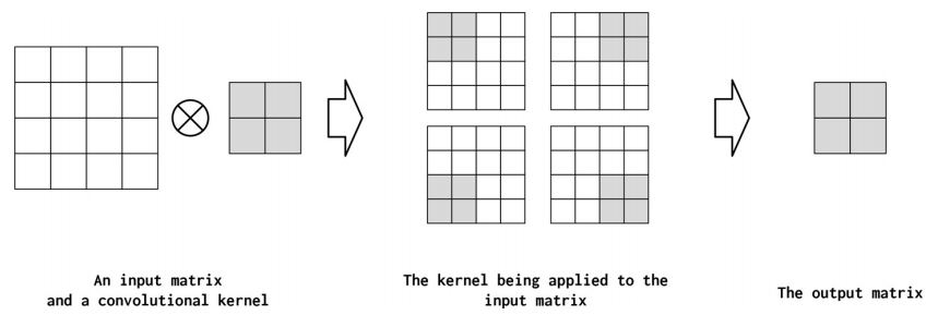
为了理解不同的设计决策对CNN意味着什么，我们在图4-6中展示了一个示例。在本例中，单个“核”应用于输入矩阵。卷积运算(线性算子)的精确数学表达式对于理解这一节并不重要，但是从这个图中可以直观地看出，核是一个小的方阵，它被系统地应用于输入矩阵的不同位置。

图4-6 二维卷积运算。

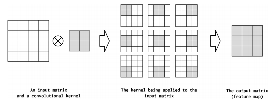
输入矩阵与单个产生输出矩阵的卷积核（也称为特征映射）在输入矩阵的每个位置应用内核。在每个应用程序中，内核乘以输入矩阵的值及其自身的值，然后将这些乘法相加kernel具有以下超参数配置：kernel_size=2，stride=1，padding=0，以及dilation=1。这些超参数解释如下:

虽然经典卷积是通过指定核的具体值来设计的，但是CNN是通过指定控制CNN行为的超参数来设计的，然后使用梯度下降来为给定数据集找到最佳参数。两个主要的超参数控制卷积的形状(称为kernel_size)和卷积将在输入数据张量(称为stride)中相乘的位置。还有一些额外的超参数控制输入数据张量被0填充了多少(称为padding)，以及当应用到输入数据张量(称为dilation)时，乘法应该相隔多远。在下面的小节中，我们将更详细地介绍这些超参数。

DIMENSION OF THE CONVOLUTION OPERATION

首先要理解的概念是卷积运算的维数。在图4-6和本节的其他图中，我们使用二维卷积进行说明，但是根据数据的性质，还有更适合的其他维度的卷积。在PyTorch中，卷积可以是一维、二维或三维的，分别由Conv1d、Conv2d和Conv3d模块实现。一维卷积对于每个时间步都有一个特征向量的时间序列非常有用。在这种情况下，我们可以在序列维度上学习模式。NLP中的卷积运算大多是一维的卷积。另一方面，二维卷积试图捕捉数据中沿两个方向的时空模式;例如，在图像中沿高度和宽度维度——为什么二维卷积在图像处理中很流行。类似地，在三维卷积中，模式是沿着数据中的三维捕获的。例如，在视频数据中，信息是三维的，二维表示图像的帧，时间维表示帧的序列。就本课程而言，我们主要使用Conv1d。

CHANNELS

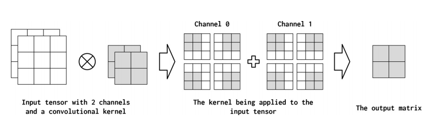
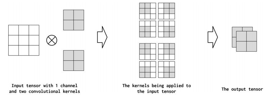
非正式地，通道(channel)是指沿输入中的每个点的特征维度。例如，在图像中，对应于RGB组件的图像中的每个像素有三个通道。在使用卷积时，文本数据也可以采用类似的概念。从概念上讲，如果文本文档中的“像素”是单词，那么通道的数量就是词汇表的大小。如果我们更细粒度地考虑字符的卷积，通道的数量就是字符集的大小(在本例中刚好是词汇表)。在PyTorch卷积实现中，输入通道的数量是in_channels参数。卷积操作可以在输出(out_channels)中产生多个通道。您可以将其视为卷积运算符将输入特征维“映射”到输出特征维。图4-7和图4-8说明了这个概念。

图4-7 卷积运算用两个输入矩阵（两个输入通道）表示相应的核也有两层，它将每层分别相乘，然后对结果求和。参数配置：input_channels=2, output_channels=1, kernel_size=2, tride=1, padding=0, and dilation=1.

图4-8 一种具有一个输入矩阵（一个输入通道）和两个卷积的卷积运算核（两个输出通道）。这些核分别应用于输入矩阵，并堆叠在输出张量。参数配置：input_channels=1, output_channels=2, kernel_size=2, tride=1, padding=0, and dilation=1.

很难立即知道有多少输出通道适合当前的问题。为了简化这个困难，我们假设边界是1,1,024——我们可以有一个只有一个通道的卷积层，也可以有一个只有1,024个通道的卷积层。现在我们有了边界，接下来要考虑的是有多少个输入通道。一种常见的设计模式是，从一个卷积层到下一个卷积层，通道数量的缩减不超过2倍。这不是一个硬性的规则，但是它应该让您了解适当数量的out_channels是什么样子的。

KERNEL SIZE

核矩阵的宽度称为核大小(PyTorch中的kernel_size)。在图4-6中，核大小为2，而在图4-9中，我们显示了一个大小为3的内核。卷积将输入中的空间(或时间)本地信息组合在一起，每个卷积的本地信息量由内核大小控制。然而，通过增加核的大小，也会减少输出的大小(Dumoulin和Visin, 2016)。这就是为什么当核大小为3时，输出矩阵是图4-9中的2x2，而当核大小为2时，输出矩阵是图4-6中的3x3。

图4-9 将kernel_size=3的卷积应用于输入矩阵。结果是一个折衷的结果：在每次将内核应用于矩阵时，都会使用更多的局部信息，但输出的大小会更小.

此外，可以将NLP应用程序中核大小的行为看作类似于通过查看单词组捕获语言模式的n-gram的行为。使用较小的核大小，可以捕获较小的频繁模式，而较大的核大小会导致较大的模式，这可能更有意义，但是发生的频率更低。较小的核大小会导致输出中的细粒度特性，而较大的核大小会导致粗粒度特性。

STRIDE

Stride控制卷积之间的步长。如果步长与核相同，则内核计算不会重叠。另一方面，如果跨度为1，则内核重叠最大。输出张量可以通过增加步幅的方式被有意的压缩来总结信息，如图4-10所示。

图4-10 应用于具有超参数步长的输入的kernel_size=2的卷积核等于2。这会导致内核采取更大的步骤，从而产生更小的输出矩阵。对于更稀疏地对输入矩阵进行二次采样非常有用。

PADDING

即使stride和kernel_size允许控制每个计算出的特征值有多大范围，它们也有一个有害的、有时是无意的副作用，那就是缩小特征映射的总大小(卷积的输出)。为了抵消这一点，输入数据张量被人为地增加了长度(如果是一维、二维或三维)、高度(如果是二维或三维)和深度(如果是三维)，方法是在每个维度上附加和前置0。这意味着CNN将执行更多的卷积，但是输出形状可以控制，而不会影响所需的核大小、步幅或扩展。图4-11展示了正在运行的填充。

图4-11 应用于高度和宽度等于的输入矩阵的kernel_size=2的卷积2。但是，由于填充（用深灰色正方形表示），输入矩阵的高度和宽度可以被放大。这通常与大小为3的内核一起使用，这样输出矩阵将等于输入矩阵的大小。

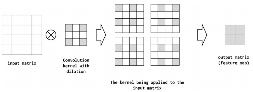
DILATION

膨胀控制卷积核如何应用于输入矩阵。在图4-12中，我们显示，将膨胀从1(默认值)增加到2意味着当应用于输入矩阵时，核的元素彼此之间是两个空格。另一种考虑这个问题的方法是在核中跨跃——在核中的元素或核的应用之间存在一个step size，即存在“holes”。这对于在不增加参数数量的情况下总结输入空间的更大区域是有用的。当卷积层被叠加时，扩张卷积被证明是非常有用的。连续扩张的卷积指数级地增大了“接受域”的大小；即网络在做出预测之前所看到的输入空间的大小。

图4-12 应用于超参数dilation=2的输入矩阵的kernel_size=2的卷积。从默认值开始膨胀的增加意味着核矩阵的元素在与输入矩阵相乘时进一步分散开来。进一步增大扩张会加剧这种扩散。

3.3 Implementing CNNs in PyTorch

在本节中，我们将通过端到端示例来利用上一节中介绍的概念。一般来说，神经网络设计的目标是找到一个能够完成任务的超参数组态。我们再次考虑在“示例:带有多层感知器的姓氏分类”中引入的现在很熟悉的姓氏分类任务，但是我们将使用CNNs而不是MLP。我们仍然需要应用最后一个线性层，它将学会从一系列卷积层创建的特征向量创建预测向量。这意味着目标是确定卷积层的配置，从而得到所需的特征向量。所有CNN应用程序都是这样的:首先有一组卷积层，它们提取一个feature map，然后将其作为上游处理的输入。在分类中，上游处理几乎总是应用线性(或fc)层。

本课程中的实现遍历设计决策，以构建一个特征向量。我们首先构造一个人工数据张量，以反映实际数据的形状。数据张量的大小是三维的——这是向量化文本数据的最小批大小。如果你对一个字符序列中的每个字符使用onehot向量，那么onehot向量序列就是一个矩阵，而onehot矩阵的小批量就是一个三维张量。使用卷积的术语，每个onehot(通常是词汇表的大小)的大小是”input channels”的数量，字符序列的长度是“width”。

在例4-14中，构造特征向量的第一步是将PyTorch的Conv1d类的一个实例应用到三维数据张量。通过检查输出的大小，你可以知道张量减少了多少。建议参考图4-9来直观地解释为什么输出张量在收缩。

Example 4-14. Artificial data and using a Conv1d class

import torch
import torch.nn as nn

batch_size = 2
one_hot_size = 10
sequence_width = 7
data = torch.randn(batch_size, one_hot_size, sequence_width)
conv1 = nn.Conv1d(in_channels=one_hot_size, out_channels=16,
               kernel_size=3)
intermediate1 = conv1(data)
print(data.size())
print(intermediate1.size())

torch.Size([2, 10, 7])
torch.Size([2, 16, 5])

进一步减小输出张量的主要方法有三种。第一种方法是创建额外的卷积并按顺序应用它们。最终，对应的sequence_width (dim=2)维度的大小将为1。我们在例4-15中展示了应用两个额外卷积的结果。一般来说，对输出张量的约简应用卷积的过程是迭代的，需要一些猜测工作。我们的示例是这样构造的:经过三次卷积之后，最终的输出在最终维度上的大小为1。

Example 4-15. The iterative application of convolutions to data

conv2 = nn.Conv1d(in_channels=16, out_channels=32, kernel_size=3)
conv3 = nn.Conv1d(in_channels=32, out_channels=64, kernel_size=3)

intermediate2 = conv2(intermediate1)
intermediate3 = conv3(intermediate2)

print(intermediate2.size())
print(intermediate3.size())

torch.Size([2, 32, 3])
torch.Size([2, 64, 1])

y_output = intermediate3.squeeze()
print(y_output.size())

torch.Size([2, 64])

在每次卷积中，通道维数的大小都会增加，因为通道维数是每个数据点的特征向量。张量实际上是一个特征向量的最后一步是去掉讨厌的尺寸=1维。您可以使用squeeze()方法来实现这一点。该方法将删除size=1的所有维度并返回结果。然后，得到的特征向量可以与其他神经网络组件(如线性层)一起使用来计算预测向量。

另外还有两种方法可以将张量简化为每个数据点的一个特征向量:将剩余的值压平为特征向量，并在额外维度上求平均值。这两种方法如示例4-16所示。使用第一种方法，只需使用PyTorch的view()方法将所有向量平展成单个向量。第二种方法使用一些数学运算来总结向量中的信息。最常见的操作是算术平均值，但沿feature map维数求和和使用最大值也是常见的。每种方法都有其优点和缺点。扁平化保留了所有的信息，但会导致比预期(或计算上可行)更大的特征向量。平均变得与额外维度的大小无关，但可能会丢失信息。

Example 4-16. Two additional methods for reducing to feature vectors

# Method 2 of reducing to feature vectors
print(intermediate1.view(batch_size, -1).size())

# Method 3 of reducing to feature vectors
print(torch.mean(intermediate1, dim=2).size())
# print(torch.max(intermediate1, dim=2).size())
# print(torch.sum(intermediate1, dim=2).size())

torch.Size([2, 80])
torch.Size([2, 16])

这种设计一系列卷积的方法是基于经验的:从数据的预期大小开始，处理一系列卷积，最终得到适合您的特征向量。虽然这种方法在实践中效果很好，但在给定卷积的超参数和输入张量的情况下，还有另一种计算张量输出大小的方法，即使用从卷积运算本身推导出的数学公式。

3.4 Example: Classifying Surnames by Using a CNN

为了证明CNN的有效性，让我们应用一个简单的CNN模型来分类姓氏。这项任务的许多细节与前面的MLP示例相同，但真正发生变化的是模型的构造和向量化过程。模型的输入，而不是我们在上一个例子中看到的收缩的onehot，将是一个onehot的矩阵。这种设计将使CNN能够更好地“view”字符的排列，并对在“示例:带有多层感知器的姓氏分类”中使用的收缩的onehot编码中丢失的序列信息进行编码。

3.4.1 The SurnameDataset

虽然姓氏数据集之前在“示例:带有多层感知器的姓氏分类”中进行了描述，但建议参考“姓氏数据集”来了解它的描述。尽管我们使用了来自“示例:带有多层感知器的姓氏分类”中的相同数据集，但在实现上有一个不同之处:数据集由onehot向量矩阵组成，而不是一个收缩的onehot向量。为此，我们实现了一个数据集类，它跟踪最长的姓氏，并将其作为矩阵中包含的行数提供给矢量化器。列的数量是onehot向量的大小(词汇表的大小)。示例4-17显示了对SurnameDataset.__getitem__的更改;我们显示对SurnameVectorizer的更改。在下一小节向量化。

我们使用数据集中最长的姓氏来控制onehot矩阵的大小有两个原因。首先，将每一小批姓氏矩阵组合成一个三维张量，要求它们的大小相同。其次，使用数据集中最长的姓氏意味着可以以相同的方式处理每个小批处理。

Example 4-17. SurnameDataset modified for passing the maximum surname length

class SurnameDataset(Dataset):
    def __init__(self, surname_df, vectorizer):
        """
        Args:
            name_df (pandas.DataFrame): the dataset
            vectorizer (SurnameVectorizer): vectorizer instatiated from dataset
        """
        self.surname_df = surname_df
        self._vectorizer = vectorizer
        self.train_df = self.surname_df[self.surname_df.split=='train']
        self.train_size = len(self.train_df)

        self.val_df = self.surname_df[self.surname_df.split=='val']
        self.validation_size = len(self.val_df)

        self.test_df = self.surname_df[self.surname_df.split=='test']
        self.test_size = len(self.test_df)

        self._lookup_dict = {'train': (self.train_df, self.train_size),
                             'val': (self.val_df, self.validation_size),
                             'test': (self.test_df, self.test_size)}

        self.set_split('train')
        
        # Class weights
        class_counts = surname_df.nationality.value_counts().to_dict()
        def sort_key(item):
            return self._vectorizer.nationality_vocab.lookup_token(item[0])
        sorted_counts = sorted(class_counts.items(), key=sort_key)
        frequencies = [count for _, count in sorted_counts]
        self.class_weights = 1.0 / torch.tensor(frequencies, dtype=torch.float32)


    @classmethod
    def load_dataset_and_make_vectorizer(cls, surname_csv):
        """Load dataset and make a new vectorizer from scratch
        
        Args:
            surname_csv (str): location of the dataset
        Returns:
            an instance of SurnameDataset
        """
        surname_df = pd.read_csv(surname_csv)
        train_surname_df = surname_df[surname_df.split=='train']
        return cls(surname_df, SurnameVectorizer.from_dataframe(train_surname_df))

    @classmethod
    def load_dataset_and_load_vectorizer(cls, surname_csv, vectorizer_filepath):
        """Load dataset and the corresponding vectorizer. 
        Used in the case in the vectorizer has been cached for re-use
        
        Args:
            surname_csv (str): location of the dataset
            vectorizer_filepath (str): location of the saved vectorizer
        Returns:
            an instance of SurnameDataset
        """
        surname_df = pd.read_csv(surname_csv)
        vectorizer = cls.load_vectorizer_only(vectorizer_filepath)
        return cls(surname_df, vectorizer)

    @staticmethod
    def load_vectorizer_only(vectorizer_filepath):
        """a static method for loading the vectorizer from file
        
        Args:
            vectorizer_filepath (str): the location of the serialized vectorizer
        Returns:
            an instance of SurnameDataset
        """
        with open(vectorizer_filepath) as fp:
            return SurnameVectorizer.from_serializable(json.load(fp))

    def save_vectorizer(self, vectorizer_filepath):
        """saves the vectorizer to disk using json
        
        Args:
            vectorizer_filepath (str): the location to save the vectorizer
        """
        with open(vectorizer_filepath, "w") as fp:
            json.dump(self._vectorizer.to_serializable(), fp)

    def get_vectorizer(self):
        """ returns the vectorizer """
        return self._vectorizer

    def set_split(self, split="train"):
        """ selects the splits in the dataset using a column in the dataframe """
        self._target_split = split
        self._target_df, self._target_size = self._lookup_dict[split]

    def __len__(self):
        return self._target_size

    def __getitem__(self, index):
        """the primary entry point method for PyTorch datasets
        
        Args:
            index (int): the index to the data point 
        Returns:
            a dictionary holding the data point's features (x_data) and label (y_target)
        """
        row = self._target_df.iloc[index]

        surname_matrix = \
            self._vectorizer.vectorize(row.surname)

        nationality_index = \
            self._vectorizer.nationality_vocab.lookup_token(row.nationality)

        return {'x_surname': surname_matrix,
                'y_nationality': nationality_index}

    def get_num_batches(self, batch_size):
        """Given a batch size, return the number of batches in the dataset
        
        Args:
            batch_size (int)
        Returns:
            number of batches in the dataset
        """
        return len(self) // batch_size

    
def generate_batches(dataset, batch_size, shuffle=True,
                     drop_last=True, device="cpu"):
    """
    A generator function which wraps the PyTorch DataLoader. It will 
      ensure each tensor is on the write device location.
    """
    dataloader = DataLoader(dataset=dataset, batch_size=batch_size,
                            shuffle=shuffle, drop_last=drop_last)

    for data_dict in dataloader:
        out_data_dict = {}
        for name, tensor in data_dict.items():
            out_data_dict[name] = data_dict[name].to(device)
        yield out_data_dict

3.4.2 Vocabulary, Vectorizer, and DataLoader

在本例中，尽管词汇表和DataLoader的实现方式与“示例:带有多层感知器的姓氏分类”中的示例相同，但Vectorizer的vectorize()方法已经更改，以适应CNN模型的需要。具体来说，正如我们在示例4-18中的代码中所示，该函数将字符串中的每个字符映射到一个整数，然后使用该整数构造一个由onehot向量组成的矩阵。重要的是，矩阵中的每一列都是不同的onehot向量。主要原因是，我们将使用的Conv1d层要求数据张量在第0维上具有批处理，在第1维上具有通道，在第2维上具有特性。

除了更改为使用onehot矩阵之外，我们还修改了矢量化器，以便计算姓氏的最大长度并将其保存为max_surname_length

Example 4-18. Implementing the Surname Vectorizer for CNNs

class SurnameVectorizer(object):
    """ The Vectorizer which coordinates the Vocabularies and puts them to use"""
    def __init__(self, surname_vocab, nationality_vocab, max_surname_length):
        """
        Args:
            surname_vocab (Vocabulary): maps characters to integers
            nationality_vocab (Vocabulary): maps nationalities to integers
            max_surname_length (int): the length of the longest surname
        """
        self.surname_vocab = surname_vocab
        self.nationality_vocab = nationality_vocab
        self._max_surname_length = max_surname_length

    def vectorize(self, surname):
        """
        Args:
            surname (str): the surname
        Returns:
            one_hot_matrix (np.ndarray): a matrix of one-hot vectors
        """

        one_hot_matrix_size = (len(self.surname_vocab), self._max_surname_length)
        one_hot_matrix = np.zeros(one_hot_matrix_size, dtype=np.float32)
                               
        for position_index, character in enumerate(surname):
            character_index = self.surname_vocab.lookup_token(character)
            one_hot_matrix[character_index][position_index] = 1
        
        return one_hot_matrix

    @classmethod
    def from_dataframe(cls, surname_df):
        """Instantiate the vectorizer from the dataset dataframe
        
        Args:
            surname_df (pandas.DataFrame): the surnames dataset
        Returns:
            an instance of the SurnameVectorizer
        """
        surname_vocab = Vocabulary(unk_token="@")
        nationality_vocab = Vocabulary(add_unk=False)
        max_surname_length = 0

        for index, row in surname_df.iterrows():
            max_surname_length = max(max_surname_length, len(row.surname))
            for letter in row.surname:
                surname_vocab.add_token(letter)
            nationality_vocab.add_token(row.nationality)

        return cls(surname_vocab, nationality_vocab, max_surname_length)

    @classmethod
    def from_serializable(cls, contents):
        surname_vocab = Vocabulary.from_serializable(contents['surname_vocab'])
        nationality_vocab =  Vocabulary.from_serializable(contents['nationality_vocab'])
        return cls(surname_vocab=surname_vocab, nationality_vocab=nationality_vocab, 
                   max_surname_length=contents['max_surname_length'])

    def to_serializable(self):
        return {'surname_vocab': self.surname_vocab.to_serializable(),
                'nationality_vocab': self.nationality_vocab.to_serializable(), 
                'max_surname_length': self._max_surname_length}

3.4.3 Reimplementing the SurnameClassifier with Convolutional Networks

我们在本例中使用的模型是使用我们在“卷积神经网络”中介绍的方法构建的。实际上，我们在该部分中创建的用于测试卷积层的“人工”数据与姓氏数据集中使用本例中的矢量化器的数据张量的大小完全匹配。正如在示例4-19中所看到的，它与我们在“卷积神经网络”中引入的Conv1d序列既有相似之处，也有需要解释的新添加内容。具体来说，该模型类似于“卷积神经网络”，它使用一系列一维卷积来增量地计算更多的特征，从而得到一个单特征向量。

然而，本例中的新内容是使用sequence和ELU PyTorch模块。序列模块是封装线性操作序列的方便包装器。在这种情况下，我们使用它来封装Conv1d序列的应用程序。ELU是类似于实验3中介绍的ReLU的非线性函数，但是它不是将值裁剪到0以下，而是对它们求幂。ELU已经被证明是卷积层之间使用的一种很有前途的非线性(Clevert et al.， 2015)。

在本例中，我们将每个卷积的通道数与num_channels超参数绑定。我们可以选择不同数量的通道分别进行卷积运算。这样做需要优化更多的超参数。我们发现256足够大，可以使模型达到合理的性能。

Example 4-19. The CNN-based SurnameClassifier

class SurnameClassifier(nn.Module):
    def __init__(self, initial_num_channels, num_classes, num_channels):
        """
        Args:
            initial_num_channels (int): size of the incoming feature vector
            num_classes (int): size of the output prediction vector
            num_channels (int): constant channel size to use throughout network
        """
        super(SurnameClassifier, self).__init__()
        
        self.convnet = nn.Sequential(
            nn.Conv1d(in_channels=initial_num_channels, 
                      out_channels=num_channels, kernel_size=3),
            nn.ELU(),
            nn.Conv1d(in_channels=num_channels, out_channels=num_channels, 
                      kernel_size=3, stride=2),
            nn.ELU(),
            nn.Conv1d(in_channels=num_channels, out_channels=num_channels, 
                      kernel_size=3, stride=2),
            nn.ELU(),
            nn.Conv1d(in_channels=num_channels, out_channels=num_channels, 
                      kernel_size=3),
            nn.ELU()
        )
        self.fc = nn.Linear(num_channels, num_classes)

    def forward(self, x_surname, apply_softmax=False):
        """The forward pass of the classifier
        
        Args:
            x_surname (torch.Tensor): an input data tensor. 
                x_surname.shape should be (batch, initial_num_channels, max_surname_length)
            apply_softmax (bool): a flag for the softmax activation
                should be false if used with the Cross Entropy losses
        Returns:
            the resulting tensor. tensor.shape should be (batch, num_classes)
        """
        features = self.convnet(x_surname).squeeze(dim=2)
       
        prediction_vector = self.fc(features)

        if apply_softmax:
            prediction_vector = F.softmax(prediction_vector, dim=1)

        return prediction_vector

3.4.4 The Training Routine

训练程序包括以下似曾相识的的操作序列:实例化数据集,实例化模型,实例化损失函数,实例化优化器,遍历数据集的训练分区和更新模型参数,遍历数据集的验证分区和测量性能,然后重复数据集迭代一定次数。此时，这是本书到目前为止的第三个训练例程实现，应该将这个操作序列内部化。对于这个例子，我们将不再详细描述具体的训练例程，因为它与“示例:带有多层感知器的姓氏分类”中的例程完全相同。但是，输入参数是不同的，可以在示例4-20中看到。

Example 4-20. Input arguments to the CNN surname classifier

args = Namespace(
    # Data and Path information
    surname_csv="data/surnames/surnames_with_splits.csv",
    vectorizer_file="vectorizer.json",
    model_state_file="model.pth",
    save_dir="model_storage/ch4/cnn",
    # Model hyper parameters
    hidden_dim=100,
    num_channels=256,
    # Training hyper parameters
    seed=1337,
    learning_rate=0.001,
    batch_size=128,
    num_epochs=100,
    early_stopping_criteria=5,
    dropout_p=0.1,
    # Runtime options
    cuda=False,
    reload_from_files=False,
    expand_filepaths_to_save_dir=True,
    catch_keyboard_interrupt=True
)


if args.expand_filepaths_to_save_dir:
    args.vectorizer_file = os.path.join(args.save_dir,
                                        args.vectorizer_file)

    args.model_state_file = os.path.join(args.save_dir,
                                         args.model_state_file)
    
    print("Expanded filepaths: ")
    print("\t{}".format(args.vectorizer_file))
    print("\t{}".format(args.model_state_file))
    
# Check CUDA
if not torch.cuda.is_available():
    args.cuda = False

args.device = torch.device("cuda" if args.cuda else "cpu")
print("Using CUDA: {}".format(args.cuda))

def set_seed_everywhere(seed, cuda):
    np.random.seed(seed)
    torch.manual_seed(seed)
    if cuda:
        torch.cuda.manual_seed_all(seed)
        
def handle_dirs(dirpath):
    if not os.path.exists(dirpath):
        os.makedirs(dirpath)
        
# Set seed for reproducibility
set_seed_everywhere(args.seed, args.cuda)

# handle dirs
handle_dirs(args.save_dir)

if args.reload_from_files:
    # training from a checkpoint
    dataset = SurnameDataset.load_dataset_and_load_vectorizer(args.surname_csv,
                                                              args.vectorizer_file)
else:
    # create dataset and vectorizer
    dataset = SurnameDataset.load_dataset_and_make_vectorizer(args.surname_csv)
    dataset.save_vectorizer(args.vectorizer_file)
    
vectorizer = dataset.get_vectorizer()

classifier = SurnameClassifier(initial_num_channels=len(vectorizer.surname_vocab), 
                               num_classes=len(vectorizer.nationality_vocab),
                               num_channels=args.num_channels)

classifer = classifier.to(args.device)
dataset.class_weights = dataset.class_weights.to(args.device)

loss_func = nn.CrossEntropyLoss(weight=dataset.class_weights)
optimizer = optim.Adam(classifier.parameters(), lr=args.learning_rate)
scheduler = optim.lr_scheduler.ReduceLROnPlateau(optimizer=optimizer,
                                           mode='min', factor=0.5,
                                           patience=1)

train_state = make_train_state(args)

epoch_bar = tqdm_notebook(desc='training routine', 
                          total=args.num_epochs,
                          position=0)

dataset.set_split('train')
train_bar = tqdm_notebook(desc='split=train',
                          total=dataset.get_num_batches(args.batch_size), 
                          position=1, 
                          leave=True)
dataset.set_split('val')
val_bar = tqdm_notebook(desc='split=val',
                        total=dataset.get_num_batches(args.batch_size), 
                        position=1, 
                        leave=True)

try:
    for epoch_index in range(args.num_epochs):
        train_state['epoch_index'] = epoch_index

        # Iterate over training dataset

        # setup: batch generator, set loss and acc to 0, set train mode on

        dataset.set_split('train')
        batch_generator = generate_batches(dataset, 
                                           batch_size=args.batch_size, 
                                           device=args.device)
        running_loss = 0.0
        running_acc = 0.0
        classifier.train()

        for batch_index, batch_dict in enumerate(batch_generator):
            # the training routine is these 5 steps:

            # --------------------------------------
            # step 1. zero the gradients
            optimizer.zero_grad()

            # step 2. compute the output
            y_pred = classifier(batch_dict['x_surname'])

            # step 3. compute the loss
            loss = loss_func(y_pred, batch_dict['y_nationality'])
            loss_t = loss.item()
            running_loss += (loss_t - running_loss) / (batch_index + 1)

            # step 4. use loss to produce gradients
            loss.backward()

            # step 5. use optimizer to take gradient step
            optimizer.step()
            # -----------------------------------------
            # compute the accuracy
            acc_t = compute_accuracy(y_pred, batch_dict['y_nationality'])
            running_acc += (acc_t - running_acc) / (batch_index + 1)

            # update bar
            train_bar.set_postfix(loss=running_loss, acc=running_acc, 
                            epoch=epoch_index)
            train_bar.update()

        train_state['train_loss'].append(running_loss)
        train_state['train_acc'].append(running_acc)

        # Iterate over val dataset

        # setup: batch generator, set loss and acc to 0; set eval mode on
        dataset.set_split('val')
        batch_generator = generate_batches(dataset, 
                                           batch_size=args.batch_size, 
                                           device=args.device)
        running_loss = 0.
        running_acc = 0.
        classifier.eval()

        for batch_index, batch_dict in enumerate(batch_generator):

            # compute the output
            y_pred =  classifier(batch_dict['x_surname'])

            # step 3. compute the loss
            loss = loss_func(y_pred, batch_dict['y_nationality'])
            loss_t = loss.item()
            running_loss += (loss_t - running_loss) / (batch_index + 1)

            # compute the accuracy
            acc_t = compute_accuracy(y_pred, batch_dict['y_nationality'])
            running_acc += (acc_t - running_acc) / (batch_index + 1)
            val_bar.set_postfix(loss=running_loss, acc=running_acc, 
                            epoch=epoch_index)
            val_bar.update()

        train_state['val_loss'].append(running_loss)
        train_state['val_acc'].append(running_acc)

        train_state = update_train_state(args=args, model=classifier,
                                         train_state=train_state)

        scheduler.step(train_state['val_loss'][-1])

        if train_state['stop_early']:
            break

        train_bar.n = 0
        val_bar.n = 0
        epoch_bar.update()
except KeyboardInterrupt:
    print("Exiting loop")

classifier.load_state_dict(torch.load(train_state['model_filename']))

classifier = classifier.to(args.device)
dataset.class_weights = dataset.class_weights.to(args.device)
loss_func = nn.CrossEntropyLoss(dataset.class_weights)

dataset.set_split('test')
batch_generator = generate_batches(dataset, 
                                   batch_size=args.batch_size, 
                                   device=args.device)
running_loss = 0.
running_acc = 0.
classifier.eval()

for batch_index, batch_dict in enumerate(batch_generator):
    # compute the output
    y_pred =  classifier(batch_dict['x_surname'])
    
    # compute the loss
    loss = loss_func(y_pred, batch_dict['y_nationality'])
    loss_t = loss.item()
    running_loss += (loss_t - running_loss) / (batch_index + 1)

    # compute the accuracy
    acc_t = compute_accuracy(y_pred, batch_dict['y_nationality'])
    running_acc += (acc_t - running_acc) / (batch_index + 1)

train_state['test_loss'] = running_loss
train_state['test_acc'] = running_acc

print("Test loss: {};".format(train_state['test_loss']))
print("Test Accuracy: {}".format(train_state['test_acc']))

3.4.5 Model Evaluation and Prediction

要理解模型的性能，需要对性能进行定量和定性的度量。下面将描述这两个度量的基本组件。建议你扩展它们，以探索该模型及其所学习到的内容。

Evaluating on the Test Dataset
正如“示例:带有多层感知器的姓氏分类”中的示例与本示例之间的训练例程没有变化一样，执行评估的代码也没有变化。总之，调用分类器的eval()方法来防止反向传播，并迭代测试数据集。与 MLP 约 50% 的性能相比，该模型的测试集性能准确率约为56%。尽管这些性能数字绝不是这些特定架构的上限，但是通过一个相对简单的CNN模型获得的改进应该足以让您在文本数据上尝试CNNs。

Classifying or retrieving top predictions for a new surname

在本例中，predict_nationality()函数的一部分发生了更改，如示例4-21所示:我们没有使用视图方法重塑新创建的数据张量以添加批处理维度，而是使用PyTorch的unsqueeze()函数在批处理应该在的位置添加大小为1的维度。相同的更改反映在predict_topk_nationality()函数中。

Example 4-21. Using the trained model to make predictions

def predict_nationality(surname, classifier, vectorizer):
    """Predict the nationality from a new surname

    Args:
        surname (str): the surname to classifier
        classifier (SurnameClassifer): an instance of the classifier
        vectorizer (SurnameVectorizer): the corresponding vectorizer
    Returns:
        a dictionary with the most likely nationality and its probability
    """
    vectorized_surname = vectorizer.vectorize(surname)
    vectorized_surname = torch.tensor(vectorized_surname).unsqueeze(0)
    result = classifier(vectorized_surname, apply_softmax=True)

    probability_values, indices = result.max(dim=1)
    index = indices.item()

    predicted_nationality = vectorizer.nationality_vocab.lookup_index(index)
    probability_value = probability_values.item()

    return {'nationality': predicted_nationality, 'probability': probability_value}

new_surname = input("Enter a surname to classify: ")
classifier = classifier.cpu()
prediction = predict_nationality(new_surname, classifier, vectorizer)
print("{} -> {} (p={:0.2f})".format(new_surname,
                                    prediction['nationality'],
                                    prediction['probability']))

Enter a surname to classify:  Ma
Ma -> Chinese (p=0.39)

def predict_topk_nationality(surname, classifier, vectorizer, k=5):
    """Predict the top K nationalities from a new surname
    
    Args:
        surname (str): the surname to classifier
        classifier (SurnameClassifer): an instance of the classifier
        vectorizer (SurnameVectorizer): the corresponding vectorizer
        k (int): the number of top nationalities to return
    Returns:
        list of dictionaries, each dictionary is a nationality and a probability
    """
    
    vectorized_surname = vectorizer.vectorize(surname)
    vectorized_surname = torch.tensor(vectorized_surname).unsqueeze(dim=0)
    prediction_vector = classifier(vectorized_surname, apply_softmax=True)
    probability_values, indices = torch.topk(prediction_vector, k=k)
    
    # returned size is 1,k
    probability_values = probability_values[0].detach().numpy()
    indices = indices[0].detach().numpy()
    
    results = []
    for kth_index in range(k):
        nationality = vectorizer.nationality_vocab.lookup_index(indices[kth_index])
        probability_value = probability_values[kth_index]
        results.append({'nationality': nationality, 
                        'probability': probability_value})
    return results

new_surname = input("Enter a surname to classify: ")

k = int(input("How many of the top predictions to see? "))
if k > len(vectorizer.nationality_vocab):
    print("Sorry! That's more than the # of nationalities we have.. defaulting you to max size :)")
    k = len(vectorizer.nationality_vocab)
    
predictions = predict_topk_nationality(new_surname, classifier, vectorizer, k=k)

print("Top {} predictions:".format(k))
print("===================")
for prediction in predictions:
    print("{} -> {} (p={:0.2f})".format(new_surname,
                                        prediction['nationality'],
                                        prediction['probability']))

Enter a surname to classify:  Ma
How many of the top predictions to see?  5

Top 5 predictions:
===================
Ma -> Chinese (p=0.39)
Ma -> Vietnamese (p=0.35)
Ma -> Korean (p=0.25)
Ma -> Arabic (p=0.00)
Ma -> Russian (p=0.00)

3.5 Miscellaneous Topics in CNNs

为了结束我们的讨论，我们概述了几个其他的主题，这些主题是CNNs的核心，但在它们的共同使用中起着主要作用。特别是，你将看到Pooling操作、batch Normalization、network-in-network connection和residual connections的描述。
3.5.1 Pooling Operation

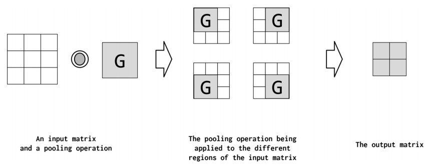
Pooling是将高维特征映射总结为低维特征映射的操作。卷积的输出是一个特征映射。feature map中的值总结了输入的一些区域。由于卷积计算的重叠性，许多计算出的特征可能是冗余的。Pooling是一种将高维(可能是冗余的)特征映射总结为低维特征映射的方法。在形式上，池是一种像sum、mean或max这样的算术运算符，系统地应用于feature map中的局部区域，得到的池操作分别称为sum pooling、average pooling和max pooling。池还可以作为一种方法，将较大但较弱的feature map的统计强度改进为较小但较强的feature map。图4-13说明了Pooling。

图4-13 这里所示的池操作在功能上与卷积相同：它应用于输入矩阵中的不同位置。然而，池操作不是将输入矩阵的值相乘和求和，而是应用一些函数G来汇集这些值。G可以是任何运算，但求和、求最大值和计算平均值是最常见的。

3.5.2 Batch Normalization (BatchNorm)

批处理标准化是设计网络时经常使用的一种工具。BatchNorm对CNN的输出进行转换，方法是将激活量缩放为零均值和单位方差。它用于Z-transform的平均值和方差值每批更新一次，这样任何单个批中的波动都不会太大地移动或影响它。BatchNorm允许模型对参数的初始化不那么敏感，并且简化了学习速率的调整(Ioffe and Szegedy, 2015)。在PyTorch中，批处理规范是在nn模块中定义的。例4-22展示了如何用卷积和线性层实例化和使用批处理规范。

Example 4-22. Using s Conv1D layer with batch normalization.

class SurnameClassifier(nn.Module):
    def __init__(self, initial_num_channels, num_classes, num_channels):
        """
        Args:
            initial_num_channels (int): size of the incoming feature vector
            num_classes (int): size of the output prediction vector
            num_channels (int): constant channel size to use throughout network
        """
        super(SurnameClassifier, self).__init__()
        
        self.convnet = nn.Sequential(
            nn.Conv1d(in_channels=initial_num_channels, 
                      out_channels=num_channels, kernel_size=3),
            nn.ELU(),
            nn.Conv1d(in_channels=num_channels, out_channels=num_channels, 
                      kernel_size=3, stride=2),
            nn.ELU(),
            nn.Conv1d(in_channels=num_channels, out_channels=num_channels, 
                      kernel_size=3, stride=2),
            nn.ELU(),
            nn.Conv1d(in_channels=num_channels, out_channels=num_channels, 
                      kernel_size=3),
            nn.ELU()
        )
        self.fc = nn.Linear(num_channels, num_classes)

    def forward(self, x_surname, apply_softmax=False):
        """The forward pass of the classifier
        
        Args:
            x_surname (torch.Tensor): an input data tensor. 
                x_surname.shape should be (batch, initial_num_channels, max_surname_length)
            apply_softmax (bool): a flag for the softmax activation
                should be false if used with the Cross Entropy losses
        Returns:
            the resulting tensor. tensor.shape should be (batch, num_classes)
        """
        features = self.convnet(x_surname).squeeze(dim=2)
       
        prediction_vector = self.fc(features)

        if apply_softmax:
            prediction_vector = F.softmax(prediction_vector, dim=1)

        return prediction_vector

3.5.3 Network-in-Network Connections (1x1 Convolutions)

Network-in-Network (NiN)连接是具有kernel_size=1的卷积内核，具有一些有趣的特性。具体来说，1x1卷积就像通道之间的一个完全连通的线性层。这在从多通道feature map映射到更浅的feature map时非常有用。在图4-14中，我们展示了一个应用于输入矩阵的NiN连接。它将两个通道简化为一个通道。因此，NiN或1x1卷积提供了一种廉价的方法来合并参数较少的额外非线性(Lin et al.， 2013)。

图4-14 一个1×1卷积运算的例子。观察1×1卷积是如何进行的操作将通道数从两个减少到一个。
3.5.4 Residual Connections/Residual Block

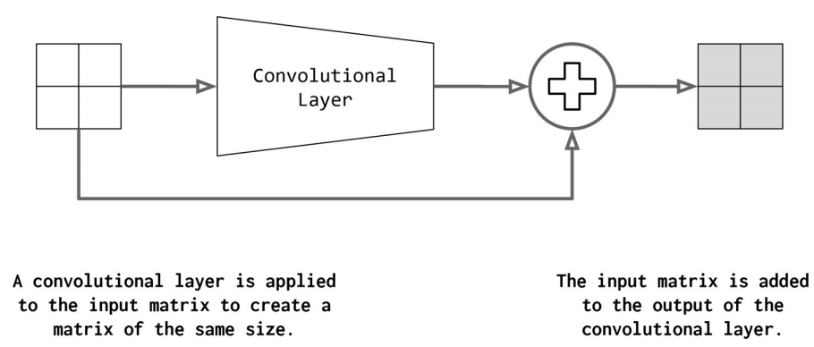
CNNs中最重要的趋势之一是Residual connection，它支持真正深层的网络(超过100层)。它也称为skip connection。如果将卷积函数表示为conv，则residual block的输出如下:

$$output=conv(input)+input$$

然而，这个操作有一个隐含的技巧，如图4-15所示。对于要添加到卷积输出的输入，它们必须具有相同的形状。为此，标准做法是在卷积之前应用填充。在图4-15中，填充尺寸为1，卷积大小为3。

图4-15 残差连接是一种将原始矩阵加到卷积输出上的方法。当将卷积层应用于输入矩阵并将结果添加到输入矩阵时，以上直观地描述了这一点。创建与输入大小相同的输出的通用超参数设置是让kernel_size=3和padding=1。一般来说，任何带 adding=(floor(kernel_size)/2-1) 的奇数内核大小都将导致与输入大小相同的输出。关于填充和卷曲的直观说明，请参见图4-11。卷积层产生的矩阵被加到输入端，最后的结果是剩余连接计算的输出端。

四、实验任务

1. 通过“示例:带有多层感知器的姓氏分类”，掌握多层感知器在多层分类中的应用

2. 掌握每种类型的神经网络层对它所计算的数据张量的大小和形状的影响

3. 尝试带有dropout的SurnameClassifier模型，看看它如何更改结果