


非线性SVM可以通过核函数构建或者自己在数据中进行构建,如若不使用核函数构建则相对于仅对数据进行变化后构建了一个线性支持向量机完成了非线性分类任务罢了,未体现SVM的高深之处,此处仅作为学习阶段的实战演练,真实运用中一般不这样
import numpy as np
from matplotlib import pyplot as plt

'''构造数据'''
X1D = np.linspace(-4, 4, 9).reshape(-1, 1)
X2D = np.c_[X1D, X1D ** 2]
y = np.array([0, 0, 1, 1, 1, 1, 1, 0, 0])
##绘图展示所绘制完成的数据
plt.figure(figsize=(11, 4))

plt.subplot(121)
plt.grid(True, which='both')
plt.axhline(y=0, color='k')
plt.plot(X1D[:, 0][y == 0], np.zeros(4), "bs")
plt.plot(X1D[:, 0][y == 1], np.zeros(5), "g")
plt.gca().get_yaxis().set_ticks([])
plt.xlabel(r"Sx_18", fontsize=20)
plt.axis([-4.5, 4.5, -0.2, 0.2])

plt.subplot(122)
plt.grid(True, which='both')
plt.axhline(y=0, color='k')
plt.axvline(x=0, color='k')
plt.plot(X2D[:, 0][y == 0], X2D[:, 1][y == 0], "bs")
plt.plot(X2D[:, 0][y == 1], X2D[:, 1][y == 1], "g^")
plt.xlabel(r"Sx_18", fontsize=20)
plt.ylabel(r"Sx_28", fontsize=20, rotation=0)
plt.gca().get_yaxis().set_ticks([0, 4, 8, 12, 16])
plt.plot([-4.5, 4.5], [6.5, 6.5], "r--", linewidtha=3)
plt.axis([-4.5, 4.5, -1, 17])
plt.subplots_adjust(right=1)
plt.show()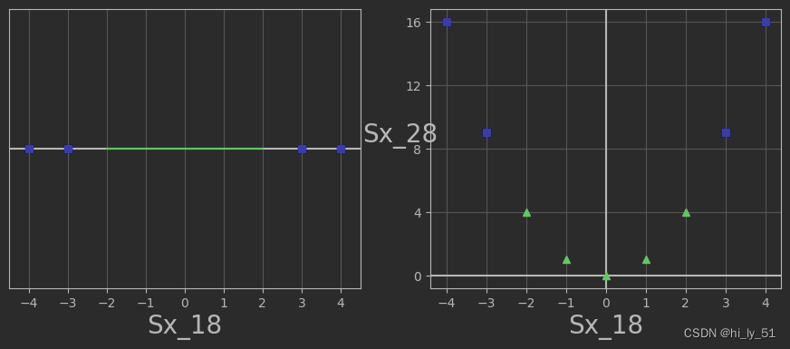
'''尝试不使用核函数的思想 直接对数据进行非线性变换'''
from sklearn.datasets import make_moons
X,y=make_moons (n_samples=100,noise=0.15,random_state=42)#指定两个环形测试数据
def plot_dataset(X,y,axes):
    plt.plot(X[:,0][y==0],X[:,1][y==0],"bs")
    plt.plot(X[:,0][y==1],X[:,1][y==1],"g^")
    plt.axis(axes)
    plt.grid(True,which='both')
    plt.xlabel(r"$x_1$",fontsize=20)
    plt.ylabel(r"$x_2$",fontsize=20,rotation=0)
plot_dataset(X,y,[-1.5,2.5,-1,1.5])
plt.show()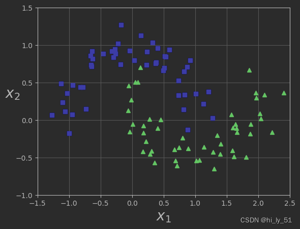
from sklearn.svm import LinearSVC
from sklearn.preprocessing import StandardScaler

'''使用SVM处理测试数据'''
from sklearn.datasets import make_moons
from sklearn.pipeline import Pipeline##使用操作流水线
from sklearn.preprocessing import PolynomialFeatures#使得特征维度增高
polynomial_svm_clf=Pipeline((("poly_features",PolynomialFeatures(degree=3)),
("scaler",StandardScaler()),
("svm_clf",LinearSVC(C=10,loss="hinge"))
))
polynomial_svm_clf.fit (X,y)
'''绘制预测结果'''
def plot_predictions(clf,axes):
    xOs=np.linspace(axes [0],axes[1],100)
    x1s=np.linspace(axes[2],axes[3],100)
    x0,x1=np.meshgrid(xOs,x1s)##构建坐标棋盘
    X=np.c_[x0.ravel(),x1.ravel()]
    y_pred =clf.predict (X).reshape(x0.shape)#一定要对预测结果进行reshape操作
    plt.contourf(x0,x1,y_pred,cmap=plt.cm.brg,alpha=0.2)

plot_predictions(polynomial_svm_clf,[-1.5,2.5,-1,1.5])
plot_dataset(X,y,[-1.5,2.5,-1,1.5])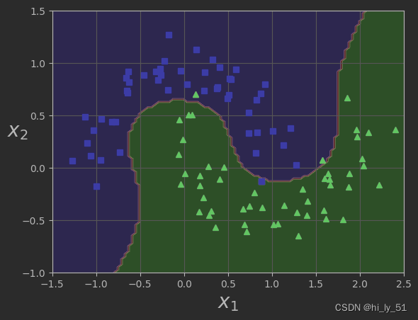


 730
730


 被折叠的 条评论
为什么被折叠?
被折叠的 条评论
为什么被折叠?
 到【灌水乐园】发言


