


特征图可视化是指将网络中某一层的特征图可视化出来,以便观察网络在不同层次上学到的特征。卷积可视化可以帮助深度学习研究者更好地理解卷积的概念和原理,从而更好地设计和优化卷积神经网络。通过可视化,研究者可以更清晰地看到卷积运算中的每一个步骤,包括输入、卷积核、卷积操作和输出,从而更好地理解卷积的本质和作用。此外,卷积可视化还可以帮助研究者更好地理解卷积神经网络中的高级概念,如池化、批量归一化等,从而更好地设计和优化深度学习模型。
本文将对卷积过程中的特征图进行可视化,研究图片经过每层卷积特征提取后,会得到哪些特征,对比观察这些特征的变化情况,能够更加熟练掌握特征图可视化操作。
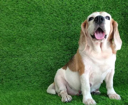
特征图可视化,这种方法是最简单,输入一张照片,然后把网络中间某层的输出的特征图按通道作为图片进行可视化展示即可。本文使用一张狗的图片进行特征图可视化。为了加快训练速度,本文仅选取一张图片进行特征图可视化,如下图1。
1、ResNet50特征图可视化
1.1 使用IntermediateLayerGetter类
# 返回输出结果
import random
import cv2
import torchvision
import torch
from matplotlib import pyplot as plt
import numpy as np
from torchvision import transforms
from torchvision import models
# 定义函数,随机从0-end的一个序列中抽取size个不同的数
def random_num(size, end):
    range_ls = [i for i in range(end)]
    num_ls = []
    for i in range(size):
        num = random.choice(range_ls)
        range_ls.remove(num)
        num_ls.append(num)
    return num_ls

path = "./input/dog.png"
transformss = transforms.Compose(
    [transforms.ToTensor(),
     transforms.Resize((224, 224)),
     transforms.Normalize([0.485, 0.456, 0.406], [0.229, 0.224, 0.225])])
# 注意如果有中文路径需要先解码,最好不要用中文
img = cv2.imread(path)
img = cv2.cvtColor(img, cv2.COLOR_BGR2RGB)
# 转换维度
img = transformss(img).unsqueeze(0)
model = models.resnet50(pretrained=True)
new_model = torchvision.models._utils.IntermediateLayerGetter(model, {'layer1': '1', 'layer2': '2', "layer3": "3"})
out = new_model(img)
tensor_ls = [(k, v) for k, v in out.items()]
# 这里选取layer2的输出画特征图
v = tensor_ls[1][1]
# 选择目标卷积层
target_layer = model.layer2[0]
"""
如果要选layer3的输出特征图只需把第一个索引值改为2,即:
v=tensor_ls[2][1]
只需把第一个索引更换为需要输出的特征层对应的位置索引即可
"""
# 取消Tensor的梯度并转成三维tensor,否则无法绘图
v = v.data.squeeze(0)
print(v.shape)  # torch.Size([512, 28, 28])
# 随机选取25个通道的特征图
channel_num = random_num(25, v.shape[0])
plt.figure(figsize=(10, 10))
for index, channel in enumerate(channel_num):
    ax = plt.subplot(5, 5, index + 1, )
    plt.imshow(v[channel, :, :])
plt.savefig("./output/feature.jpg", dpi=600)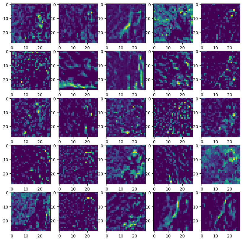
for index, channel in enumerate(channel_num):
    ax = plt.subplot(5, 5, index + 1, )
    plt.imshow(v[channel, :, :])
plt.savefig("./output/feature.jpg", dpi=600,cmap="gray") #加上cmap参数就可以显示灰度图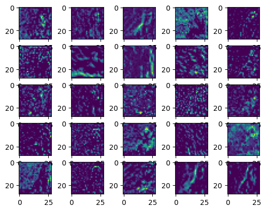
IntermediateLayerGetter有一个不足就是它不能获取二级层的输出,比如ResNet的layer2,他不能获取layer2里面的卷积的输出。
模型地址:C:\Users\Administrator\.cache\torch\hub\checkpoints
1.2 使用hook机制(推荐)
# 返回输出结果
import random

import cv2
import torchvision
import torch
from matplotlib import pyplot as plt
import numpy as np
from torchvision import transforms
from torchvision import models

# 定义函数,随机从0-end的一个序列中抽取size个不同的数
def random_num(size, end):
    range_ls = [i for i in range(end)]
    num_ls = []
    for i in range(size):
        num = random.choice(range_ls)
        range_ls.remove(num)
        num_ls.append(num)
    return num_ls


path = "./input/dog.png"
transformss = transforms.Compose(
    [transforms.ToTensor(),
     transforms.Resize((224, 224)),
     transforms.Normalize([0.485, 0.456, 0.406], [0.229, 0.224, 0.225])])

# 注意如果有中文路径需要先解码,最好不要用中文
img = cv2.imread(path)
img = cv2.cvtColor(img, cv2.COLOR_BGR2RGB)

# 转换维度
img = transformss(img).unsqueeze(0)

model = models.resnet50(pretrained=True)

# 选择目标层
target_layer = model.layer2[2]
# 注册钩子函数,用于获取目标卷积层的输出
outputs = []
def hook(module, input, output):
    outputs.append(output)

hook_handle = target_layer.register_forward_hook(hook)

_ = model(img)

v = outputs[-1]

"""
如果要选layer3的输出特征图只需把第一个索引值改为2,即:
v=tensor_ls[2][1]
只需把第一个索引更换为需要输出的特征层对应的位置索引即可
"""
# 取消Tensor的梯度并转成三维tensor,否则无法绘图
v = v.data.squeeze(0)

print(v.shape)  # torch.Size([512, 28, 28])

# 随机选取25个通道的特征图
channel_num = random_num(25, v.shape[0])
plt.figure(figsize=(10, 10))
for index, channel in enumerate(channel_num):
    ax = plt.subplot(5, 5, index + 1, )
    plt.imshow(v[channel, :, :])
plt.savefig("./output/feature2.jpg", dpi=600)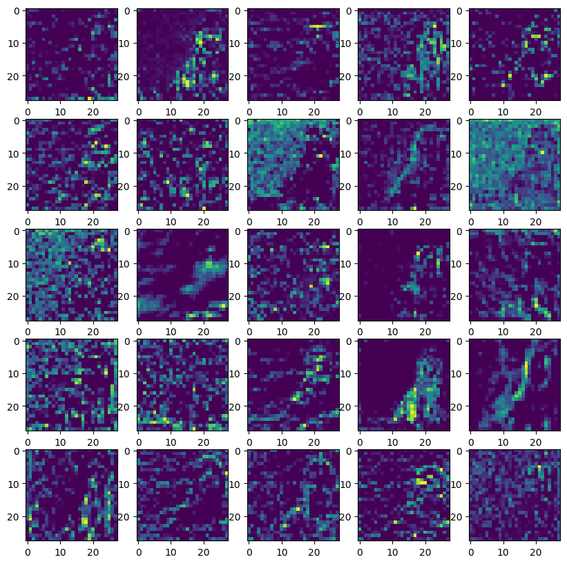
for index, channel in enumerate(channel_num):
    ax = plt.subplot(5, 5, index + 1, )
    plt.imshow(v[channel, :, :],cmap="gray")
plt.savefig("./output/feature2.jpg", dpi=600)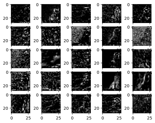
2、AlexNet特征图可视化
上面的ResNet用的是预训练模型,这里我们自己构建AlexNet
from torch import nn

class AlexNet(nn.Module):
    def __init__(self):
        super(AlexNet, self).__init__()

        self.conv1 = nn.Sequential(nn.Conv2d(3, 96, 11, 4, 2),
                                   nn.ReLU(),
                                   nn.MaxPool2d(3, 2),
                                   )

        self.conv2 = nn.Sequential(nn.Conv2d(96, 256, 5, 1, 2),
                                   nn.ReLU(),
                                   nn.MaxPool2d(3, 2),
                                   )

        self.conv3 = nn.Sequential(nn.Conv2d(256, 384, 3, 1, 1),
                                   nn.ReLU(),
                                   nn.Conv2d(384, 384, 3, 1, 1),
                                   nn.ReLU(),
                                   nn.Conv2d(384, 256, 3, 1, 1),
                                   nn.ReLU(),
                                   nn.MaxPool2d(3, 2))


        self.fc=nn.Sequential(nn.Linear(256*6*6, 4096),
                                nn.ReLU(),
                                nn.Dropout(0.5),
                                nn.Linear(4096, 4096),
                                nn.ReLU(),
                                nn.Dropout(0.5),
                                nn.Linear(4096, 100),
                                )

    def forward(self, x):
        x=self.conv1(x)
        x=self.conv2(x)
        x=self.conv3(x)
        output=self.fc(x.view(-1, 256*6*6))
        return output

model=AlexNet()
for name in model.named_children():
    print(name[0])
#同理先看网络结构
#输出
path = "./input/dog.png"
transformss = transforms.Compose(
    [transforms.ToTensor(),
     transforms.Resize((224, 224)),
     transforms.Normalize([0.485, 0.456, 0.406], [0.229, 0.224, 0.225])])

#注意如果有中文路径需要先解码,最好不要用中文
img = cv2.imread(path)
img = cv2.cvtColor(img, cv2.COLOR_BGR2RGB)

#转换维度
img = transformss(img).unsqueeze(0)

model = AlexNet()

## 修改这里传入的字典即可

new_model = torchvision.models._utils.IntermediateLayerGetter(model, {"conv1":1,"conv2":2,"conv3":3})
out = new_model(img)

tensor_ls=[(k,v) for  k,v in out.items()]

#选取conv2的输出
v=tensor_ls[1][1]

#取消Tensor的梯度并转成三维tensor,否则无法绘图
v=v.data.squeeze(0)

print(v.shape)  # torch.Size([512, 28, 28])

#随机选取25个通道的特征图
channel_num = random_num(25,v.shape[0])
plt.figure(figsize=(10, 10))
for index, channel in enumerate(channel_num):
    ax = plt.subplot(5, 5, index+1,)
    plt.imshow(v[channel, :, :])  # 灰度图参数cmap="gray"
plt.savefig("./output/feature.jpg",dpi=300)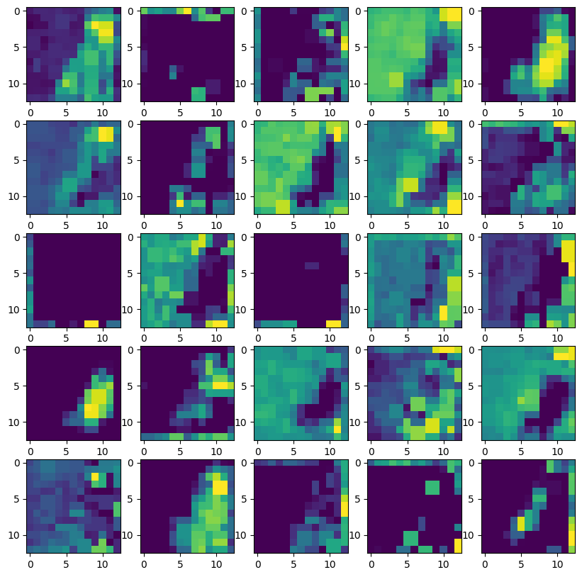
也就是说AlexNet这里分为了4部分,三个卷积和一个全连接(其实就是我们自己定义的foward前向传播),我们想要哪层的输出改个字典就好了
new_model = torchvision.models._utils.IntermediateLayerGetter(model, {“conv1”:1,“conv2”:2,“conv3”:3})
plt.imshow(v[channel, :, :],cmap=“gray”) 加上cmap参数就可以显示灰度图
for index, channel in enumerate(channel_num):
    ax = plt.subplot(5, 5, index+1,)
    plt.imshow(v[channel, :, :],cmap="gray")  # 灰度图参数cmap="gray"
plt.savefig("./output/feature.jpg",dpi=300)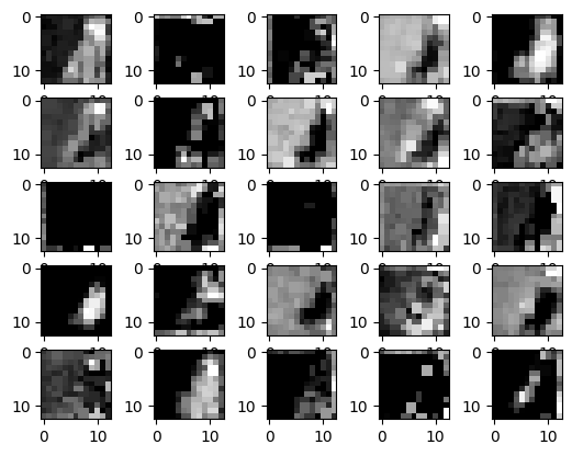
3、简易网络特征图可视化
from torch import nn
import torch
from torch.nn import functional as F
import cv2
from matplotlib import pyplot as plt

class Net(nn.Module):
    def __init__(self):
        super().__init__()
        self.conv1 = nn.Conv2d(3, 6, 5)
        self.pool1 = nn.MaxPool2d(4, 4)
        self.conv2 = nn.Conv2d(6, 16, 5)
        self.pool2 = nn.MaxPool2d(4, 4)

    def forward(self, x):
        output = []  # 保存特征层的列表,在最后的时候返回
        x = self.conv1(x)
        output.append(x)  # 加入output中
        x = F.relu(x)
        output.append(x)
        x = self.pool1(x)
        output.append(x)
        x = self.conv2(x)
        output.append(x)
        x = F.relu(x)
        output.append(x)
        x = self.pool2(x)
        return x, output

net = Net()

path = "./input/dog.png"
img = cv2.imread(path)
img = cv2.cvtColor(img, cv2.COLOR_BGR2RGB)
img = torch.tensor(img, dtype=torch.float32) / 255.0  # Normalize to [0, 1]
img = img.unsqueeze(0)  # 添加批次维度
img = img.permute(0, 3, 1, 2)  # 更改尺寸顺序
print(img.shape)

_, output = net(img)

# 打印并可视化图层
for layer in output:
    fig = plt.figure(figsize=(15, 5))  # 定义图形大小
    for i in range(layer.shape[1]):  # 迭代通道
        ax = fig.add_subplot(1, layer.shape[1], i + 1, xticks=[], yticks=[])  # 1 行,通道列数
        plt.imshow(layer[0, i].detach().numpy(), cmap="gray")  # 将通道显示为灰度图像
    plt.show()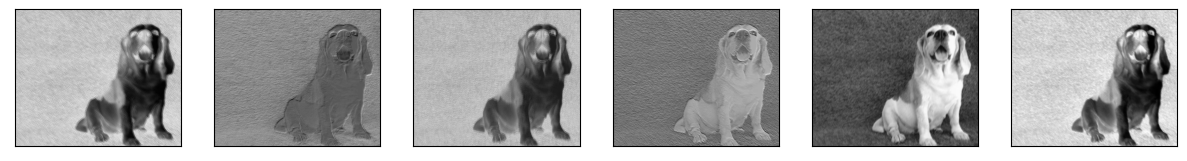


4、Yolo网络特征图可视化
import matplotlib.pyplot as plt
import torch
import torch.nn as nn
from torch.nn import functional as F
from torchvision import transforms
from PIL import Image
from net.yolov4 import YoloBody  # Assuming YoloBody is defined in yolov4.py
import cv2

# Define the hook function to get activations
activation = {}  # Save the obtained output

def get_activation(name):
    def hook(model, input, output):
        activation[name] = output.detach()
    return hook

def main():
    anchors_mask = [[6, 7, 8], [3, 4, 5], [0, 1, 2]]
    # Call the model
    model = YoloBody(3, 20)  # Assuming 3 anchors and 20 classes
    model.eval()
    # 输出网络
    for name, param in model.named_parameters():
        print(name, param.shape)

    # 在特定层上前向钩子
    model.backbone.conv1.conv.register_forward_hook(get_activation('conv'))

    # 虚拟输入图像
    x = torch.randn(1, 3, 416, 416)

    # 获取模型预测结果(可能需要根据模型结构进行修改)
    _, _, _ = model(x)

    # 从挂钩中读取激活信息
    bn = activation['conv']
    print(bn.shape)

    # 显示特征图
    plt.figure(figsize=(12, 12))
    for i in range(bn.shape[1]):
        plt.subplot(8, 8, i + 1)
        plt.imshow(bn[0, i, :, :].cpu().numpy(), cmap='gray')
        plt.axis('off')
    plt.show()
    return 0

if __name__ == '__main__':
    transform = transforms.Compose([
        transforms.Resize([416, 416]),
        transforms.ToTensor(),
        transforms.Normalize([0.485, 0.456, 0.406], [0.229, 0.224, 0.225])
    ])

    # 加载并预处理图像
    img_path = './input/dog.png'
    img = Image.open(img_path)
    input_img = transform(img).unsqueeze(0)

    print(input_img.shape)
    main()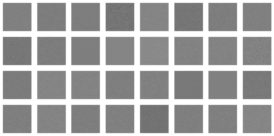
报错net的问题解决方案:zhanggong0564/YOLOV3 at d94c249d8d9ec532d2f6cff1a2be183a987c2c7f (github.com)
解决文件在YOLOV3/nets,将nets文件copy放在项目根目录下面,重命名为net即可解决。
from pathlib import Path
from pooch.utils import LOGGER
import torch
import math
import matplotlib.pyplot as plt
import numpy as np

def feature_visualization(x, module_type, stage, n=2, save_dir=Path('./output')):
    """
    x:              Features to be visualized
    module_type:    Module type
    stage:          Module stage within the model
    n:              Maximum number of feature maps to plot
    save_dir:       Directory to save results
    """
    print(f"save_dir: {save_dir}")
    if 'Detect' not in module_type:
        batch, channels, height, width = x.shape  # batch, channels, height, width
        print(f"x.shape: {x.shape}")
        if height > 1 and width > 1:
            save_dir.mkdir(parents=True, exist_ok=True)  # Ensure the directory exists

            f = save_dir / f"stage{stage}_{module_type.split('.')[-1]}_features.png"  # filename
            print(f"f: {f}")

            blocks = torch.chunk(x[0].cpu(), channels, dim=0)  # select batch index 0, block by channels
            n = min(n, channels)  # number of plots
            fig, ax = plt.subplots(math.ceil(n / 2), 2, tight_layout=True)  # 8 rows x n/8 cols
            ax = ax.ravel()
            plt.subplots_adjust(wspace=0.05, hspace=0.05)
            for i in range(n):
                ax[i].imshow(blocks[i].squeeze(), cmap='gray')  # Add cmap='gray'
                ax[i].axis('off')

            LOGGER.info(f'Saving {f}... ({n}/{channels})')
            plt.savefig(f, dpi=300, bbox_inches='tight')
            plt.close()
            np.save(str(f.with_suffix('.npy')), x[0].cpu().numpy())  # npy save
5、VGGNet特征图可视化
VGG19本是用来进行分类的,进行可视化和用作VGG loss 自然也就是用到全连接层之前的内容,先要了解VGG19全连接层之前的结构
from torchvision.models import vgg19,vgg16
import torch
import torch.nn.functional as F
device = torch.device("cuda" if torch.cuda.is_available() else "cpu")

#对于torch 的models就已经包含了vgg19
#在这里pretrained=False,在下面我自己进行了模型预加载,选择Ture,则电脑联网时
#自动会完成下载
vgg_model = vgg19(pretrained=False).features[:].to(device)
print(vgg_model)
加载vgg model
import torch
from torchvision import models

# 定义 VGG19 模型
vgg_model = models.vgg19(pretrained=True)

# 将权重保存到文件中
torch.save(vgg_model.state_dict(), 'vgg19-dcbb9e9d.pth')

# 以 strict=False 加载预训练的权重
vgg_model.load_state_dict(torch.load('vgg19-dcbb9e9d.pth'), strict=False)
vgg_model.eval()

# 将所有参数的 requires_grad 设置为 False
for param in vgg_model.parameters():
    param.requires_grad = False
模型地址 C:\Users\Administrator/.cache\torch\hub\checkpoints\vgg19-dcbb9e9d.pth
可视化
import numpy as np
import matplotlib.pyplot as plt
def get_row_col(num_maps):
    # 根据特征地图的数量计算子地图行数和列数的函数
    rows = int(np.sqrt(num_maps))
    cols = int(np.ceil(num_maps / rows))
    return rows, cols
#输入的应该时feature_maps.shape = (H,W,Channels)
#下图对relu1_2 进行了可视化,有64channels,拼了个了8*8的图
def visualize_feature_map(feature_maps):
    #创建特征子图,创建叠加后的特征图
    #param feature_batch: 一个卷积层所有特征图
    # np.squeeze(feature_maps, axis=0)
    print("visualize_feature_map shape:{},dtype:{}".format(feature_maps.shape,feature_maps.dtype))
    num_maps = feature_maps.shape[2]
    feature_map_combination = []
    plt.figure(figsize=(8, 7))
    # 取出 featurn map 的数量,因为特征图数量很多,这里直接手动指定了。
    #num_pic = feature_map.shape[2]
    row, col = get_row_col(num_maps)
    # 将 每一层卷积的特征图,拼接层 5 × 5
    for i in range(0, num_maps):
        feature_map_split = feature_maps[:, :, i]
        feature_map_combination.append(feature_map_split)
        plt.subplot(row, col, i+1)
        plt.imshow(feature_map_split)
        plt.axis('off')

    plt.savefig('./output/relu1_2_feature_map.png') # 保存图像到本地
    plt.show()
feature_maps = np.random.rand(8, 8, 64)
visualize_feature_map(feature_maps)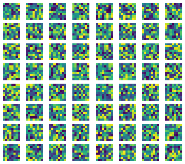
参考文献:
基于pytorch使用特征图输出进行特征图可视化-CSDN博客
【Pytorch】 特征图的可视化_pytorch 特征图可视化-CSDN博客
深度学习——pytorch卷积神经网络中间特征层可视化_pytorch获取卷积神经网络中间层-CSDN博客
Pytorch 深度学习特征图可视化——(Yolo网络、rcnn)_basicconv-CSDN博客
zhanggong0564/YOLOV3 at d94c249d8d9ec532d2f6cff1a2be183a987c2c7f (github.com)


 1384
1384

 被折叠的 条评论
为什么被折叠?
被折叠的 条评论
为什么被折叠?
 到【灌水乐园】发言


