具有模态指标的随机子空间识别【包括一致模态指标和模态参与因子】（Matlab代码实现）

wlz249

于 2024-07-19 16:03:02 发布

阅读量282

点赞数 7

文章标签： matlab 开发语言

本文链接：https://blog.csdn.net/weixin_66436111/article/details/140552513

版权

👨‍🎓个人主页：研学社的博客

💥💥💞💞欢迎来到本博客❤️❤️💥💥

🏆博主优势：🌞🌞🌞博客内容尽量做到思维缜密，逻辑清晰，为了方便读者。

⛳️座右铭：行百里者，半于九十。

📋📋📋本文目录如下：🎁🎁🎁

目录

💥1 概述

一致模态指标 (CMI)

模态参与因子 (MPF)

随机子空间识别与模态分析的结合

📚2 运行结果

🎉3 参考文献

🌈4 Matlab代码实现

💥1 概述

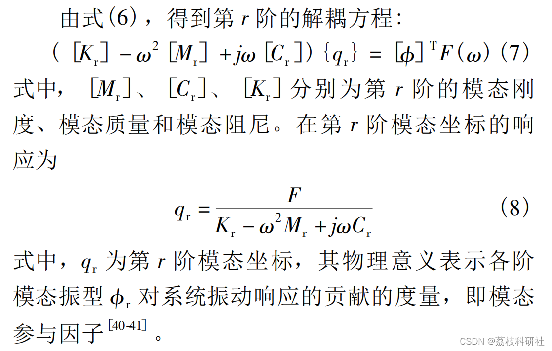
BSRMWR 可等效为一个多自由度系统，对于多自由度振动系统，其动力学方程为

$[M]\{\ddot{x}\}+[C]\{\dot{x}\}+[K]\{x\}=\{F(t)\}$

其中［M］、［C］、［K］分别表示系统质量矩阵、阻尼矩阵和刚度矩阵，三者皆为实对称矩阵。{ ·· x } 、 { · x} 、{ x} 分别表示加速度、速度和位移向量。{ F ( t) } 表示系统激励力。令{ F( t) } = { F} e jωt ，{ x} = { X} e jωt ，得:

$\left([K]-\omega^{2}[M]+j \omega[C]\right)\{X(\omega)\}=\{F(\omega)\}$

由于矩阵［M］、［C］和［K］中存在非零的非对角元素，因此式( 2) 是一组具有耦合项的方程组。运用模态矩阵作为变换矩阵，可进行坐标变换。其中模态矩阵和模态坐标如式( 3) 和( 4) 所示。

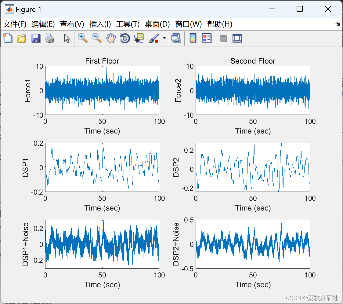
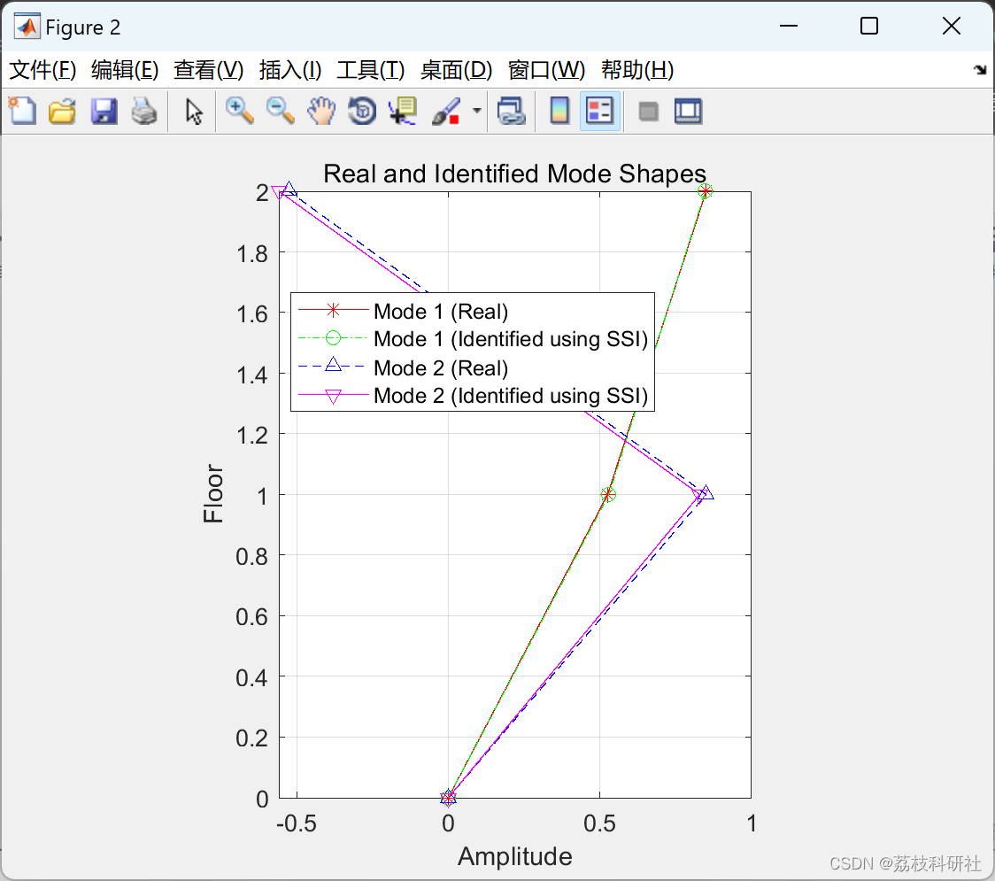
本文用于识别受高斯白噪声激励影响的2DOF系统，并增加激励和响应的不确定性（也是高斯白噪声）。

指标.EMAC ：扩展模态幅度相干
指标.MPC ：模态相位共线性
指标.CMI ：一致模式指示指标
partfac ：参与因子

随机子空间识别（Random Subspace Method, RSM）是一种机器学习方法，主要用于增强 ensemble 学习中的多样性，通过在不同的子空间上构建多个基学习器（例如决策树、支持向量机等），然后综合它们的预测来提升整体的预测性能。在处理高维数据时，RSM 能够有效避免过拟合并提高模型的泛化能力。

当涉及到模态指标，特别是“一致模态指标”（Consistent Modal Indicators, CMI）和“模态参与因子”（Modal Participation Factors, MPF）时，我们通常是在讨论模态分析领域，这与结构动力学、振动分析等相关，而非直接与随机子空间识别这一机器学习方法相关联。但我们可以尝试将这两个概念放在一起，探讨如何在结构健康监测、信号处理等领域运用随机子空间识别与模态参数分析的方法。

一致模态指标 (CMI)

在结构动力学中，一致模态指标通常用于评估结构振动响应数据中特定模态的贡献程度。它提供了一种量化特定频率范围内模态活动的方法，帮助识别和分离系统的主要振动模式。CMI 可以用于判断在某个频段内，某个模态是否被清晰地激发或是否与其他模态重叠。

模态参与因子 (MPF)

模态参与因子是描述结构各自由度在某一特定模态振动下的相对重要性的量，反映了结构各个部分对于该模态振动的贡献程度。简单来说，MPF 描述了某一模态下每个节点或自由度的振动幅值相对于整体模态振型的比值。高MPF值表明对应节点在该模态振动中起着主导作用。

随机子空间识别与模态分析的结合

虽然RSM本身不是模态分析的传统工具，但在处理大量传感器数据（如来自桥梁、建筑物的振动监测数据）进行模态参数识别时，RSM可以发挥作用。具体应用方式可能包括：

特征降维与模态提取：通过在不同随机选取的子空间上执行主成分分析（PCA）、奇异值分解（SVD）等，可以有效降低数据维度，并突出显示与特定模态相关的主成分，从而辅助模态参数的识别。
多模型集成：构建多个基于不同子集特征的基学习器来识别模态参数（如固有频率、阻尼比、模态形状），最终通过投票或平均等策略综合各个模型的输出，以提高识别精度和稳健性。
噪声抑制与特征增强：在高度嘈杂的数据环境中，随机选择的子空间可以帮助过滤掉不相关的噪声特征，强化与感兴趣模态相关的信号，从而提高模态参数估计的准确性。

综上所述，虽然CMI和MPF直接关联于结构动力学中的模态分析，而随机子空间识别属于机器学习范畴，但在处理大规模、高维的振动监测数据时，两者结合使用可以为模态识别和参数估计提供一种新颖且有效的策略，尤其是在面对复杂结构或环境噪声影响较大的情形下。

📚2 运行结果

部分代码：

function [Result]=SSID(output,fs,ncols,nrows,cut)

%Input:
%output: output data of size (No. output channels, No. of data)
%fs: Sampling frequency
%ncols: The number of columns in hankel matrix (more than 2/3 of No. of data)
%nows: The number of rows in hankel matrix (more than 20 * number of modes)
%cut: cutoff value=2*no of modes

%Outputs :
%Result : A structure consist of the below components

%Parameters.NaFreq : Natural frequencies vector
%Parameters.DampRatio : Damping ratios vector
%Parameters.ModeShape : Mode shape matrix

%Indicators.EMAC : Extended Modal Amplitude Coherence
%Indicators.MPC : Modal Phase Collinearity
%Indicators.CMI : Consistent Mode Indicator
%Indicators.partfac : Participation factor

%Matrices A,C: Discrete A and C matrices
%--------------------------------------------------------------------------

[outputs,npts]=size(output); % Computes the size of matrix output

if outputs > npts % Check if output matrix size is proper or should be transposed
output=output';
[outputs,npts]=size(output);
end

%--------------------------------------------------------------------------
% Find block sizes

brows=fix(nrows/outputs); % brows = how many output blocks.
nrows=outputs*brows; % Redefine the row numbers.
bcols=fix(ncols/1); % bcols = how many time steps.
ncols=1*bcols; % Redefine the column numbers.
m=1; % inputs number.
q=outputs; % outputs number.

%--------------------------------------------------------------------------
% Form the Hankel matriices Yp,Yf.

Yp=zeros(nrows/2,ncols); %Past Output
Yf=zeros(nrows/2,ncols); %Future Output

for ii=1:brows/2
for jj=1:bcols
Yp([(ii-1)*q+1:ii*q] ,[(jj-1)*m+1:jj*m] )=output(:,((jj-1)+ii-1)*m+1:((jj)+ii-1)*m);
end
end

for ii=brows/2+1:brows
i=ii-brows/2;
for jj=1:bcols
Yf([(i-1)*q+1:i*q] ,[(jj-1)*m+1:jj*m] )=output(:,((jj-1)+ii-1)*m+1:((jj)+ii-1)*m);
end
end

%--------------------------------------------------------------------------
% Projection
O=Yf*Yp'*pinv(Yp*Yp')*Yp;

%--------------------------------------------------------------------------
% Decompose the data matrix

[R1,Sigma1,S1]=svd(O,0);
sv=diag(Sigma1);

%--------------------------------------------------------------------------
% Truncate the matrices using the cutoff

D=diag(sqrt(sv(1:cut))); % build square root of the singular values.
Dinv=inv(D); % (sigma)^(-1/2)
Rn=R1(:,1:cut); % use only the principal eigenvectors
Sn=S1(:,1:cut); % use only the principal eigenvectors

Obs=Rn*D; % Observability matrix

%--------------------------------------------------------------------------
% Calculate the realization of A and find eigenvalues and eigenvectors

A=pinv(Obs(1:nrows/2-q,:))*Obs(q+1:nrows/2,:); % build A
C=Obs(1:q,:); % build C
clear Yp Yf;

%--------------------------------------------------------------------------
% Extract the modal frequencis , damping ratios and natural frequencis

[Vectors,Values]=eig(A); % Eigenvalues and Eigenvectors
Lambda=diag(Values); % roots in the Z-plane
s=log(Lambda).*fs; % Laplace roots
zeta=-real(s)./abs(s)*100; % damping ratios
fd=(imag(s)./2./pi);
% damped natural freqs:
shapes=C*Vectors; % Mode shapes.

%--------------------------------------------------------------------------
% Calculate Modal Participation factors

InvV=inv(Vectors);
partfac=std((InvV*D*Sn')')'; %InvV involved in transforming states to the modal amplitudes by uncoupling A matrix
%--------------------------------------------------------------------------
% Calculate EMAC values

partoutput22=(C*A^(brows/2-1)*Vectors)'; %Predicted Last Block in Obs*Vectors Matrix
partoutput2=(Rn(nrows/2-q+1:nrows/2,:)*D*Vectors)'; %Actual Last Block in Obs*Vectors Matrix (Vectors involved in transforming states to the modal amplitudes by uncoupling A matrixx)
for i=1:1:cut

sum1=0;
sum2=0;

for k=1:1:q

Rik=abs(partoutput22(i,k))/abs(partoutput2(i,k));

if Rik>1
Rik=1/Rik;
end

Wik=1-(4/pi)*abs(angle(partoutput22(i,k)/partoutput2(i,k)));

if Wik<0
Wik=0;
end

EMACout=Rik*Wik;

EMACijk=EMACout;
sum1=sum1+EMACijk*(abs(partoutput2(i,k)))^2*100;
sum2=sum2+(abs(partoutput2(i,k)))^2;
end

EMACC(i)=sum1/sum2;
end

%--------------------------------------------------------------------------
% Calculate MPC values

🎉3 参考文献

部分理论来源于网络，如有侵权请联系删除。

[1]朱伟明,杨艳,刘泽远,刘程子.基于模态参与因子的无轴承开关磁阻电机振动分析与抑制[J].微电机,2022,55(10):8-15.DOI:10.15934/j.cnki.micromotors.2022.10.001.

[2]熊笑雷,赵鸣.应变模态指标在平板网架结构损伤识别分析中的应用[J].结构工程师,2012,28(02):58-65.DOI:10.15935/j.cnki.jggcs.2012.02.012.

[3] Van Overschee, Peter, and B. L. De Moor. Subspace identification for linear systems: Theory—Implementation—Applications. Springer Science & Business Media, 2012.

[4] R. Pappa, K. Elliott, and A. Schenk, “A consistent-mode indicator for the eigensystem realization algorithm,” Journal of Guidance Control and Dynamics (1993), 1993.

[5] Al Rumaithi, Ayad, "Characterization of Dynamic Structures Using Parametric and Non-parametric System Identification Methods" (2014). Electronic Theses and Dissertations. 1325.

🌈4 Matlab代码实现

wlz249

关注

7
点赞
踩
6

收藏

觉得还不错? 一键收藏
0
评论
具有模态指标的随机子空间识别【包括一致模态指标和模态参与因子】（Matlab代码实现）

BSRMWR 可等效为一个多自由度系统，对于多自由度振动系统，其动力学方程为其中［M］、［C］、［K］分别表示系统质量矩阵、阻尼矩阵和刚度矩阵，三者皆为实对称矩阵。{ ·· x } 、 { · x} 、{ x} 分别表示加速度、速度和位移向量。{ F ( t) } 表示系统激励力。令{ F( t) } = { F} e jωt ，{ x} = { X} e jωt ，得:由于矩阵［M］、［C］和［K］中存在非零的非对角元素，因此式( 2) 是一组具有耦合项的方程组。
复制链接

扫一扫