微博FiBiNET: Combining Feature Importance and Bilinear feature Interaction for CTR Prediction

FiBiNET: Combining Feature Importance and Bilinear feature Interaction for Click-Through Rate Prediction

重点回顾下这篇论文中筛选重要特征的经典做法SeNet。

提出背景

之前的一些工作聚焦在特征交叉上面，像Hadamard product、Inner product，对特征重要性关注较少。

其实SeNet的做法就是对特征做attention操作，动态找出重要的特征，可以说是判别特征重要性的神器。

实际的推荐系统，有大量的特征Embedding因为样本数据极度稀疏，没法学习的很好比如大量低活用户的ID特征、大量长尾的物料ID特征、长尾的一些tag特征等，他们出现的次数很少，想要学习出一个靠谱的Embedding几乎不可能。如果我们一股脑把所有特征都作为输入塞进炼丹炉，那必然会引入噪音导致推荐效果不佳。在炼丹之前，如果能对炼丹材料各个特征Embedding进行挑选，对特征Embedding做重要性打分，然后根据重要程度来加大重要的特征的权重输入，同时抑制不重要特征的输入，效果必然会有所提升。

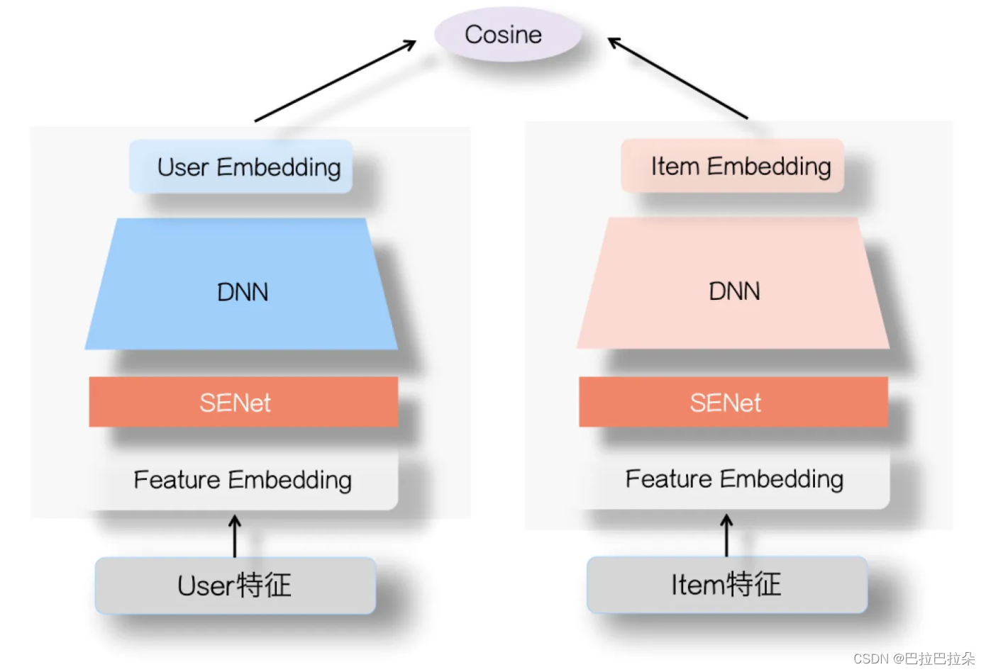
以DSSM双塔为例，SeNet的结构如下：

详细做法

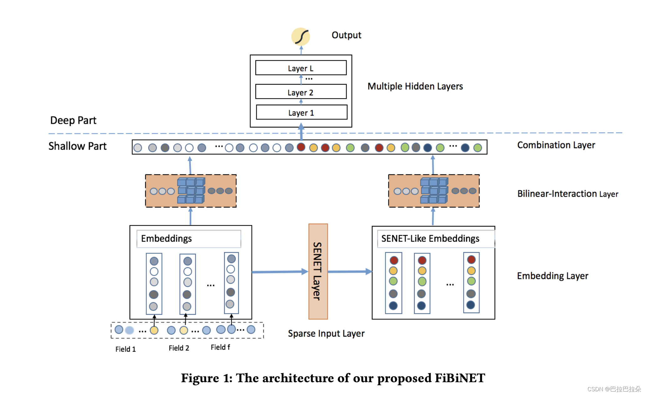
整体结构如下

其中的SENet结构如下

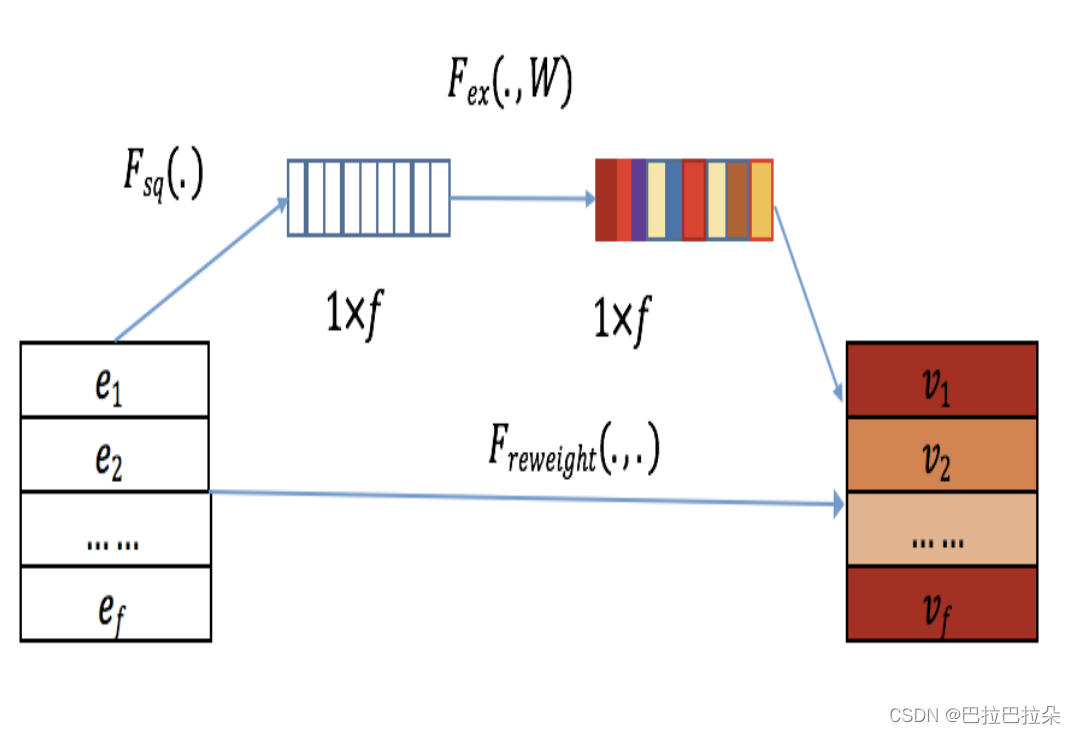
分为三步，整体是用两个全连接层操作（不过实际运用可以只用一个）

Squeeze

用户的$f$个特征对应的Embedding集合$\mathbf{E}=({\mathbf{e}}_1,{\mathbf{e}}_2,...,{\mathbf{e}}_f{)}^T\in R^{f\times d}$，讲每个特征Embedding取平均，相当于取到代表每个特征Embedding的精华
$$z_i=F_{squeeze}({\mathbf{e}}_i)=\sum _{j=1}^k{e}_{ij}$$
得到向量$\mathbf{z}=[z_1,z_2,....,z_f]$

Excitation

对每个特征的精华值进行非线性变换，得到每个特征的重要性得分
$$\mathbf{a}=F_{excitation}(\mathbf{z})={\sigma }_2({\mathbf{W}}_2{\sigma }_1({\mathbf{W}}_1\mathbf{z}))$$

Re-Weight

根据重要性对特征Embedding做attention操作
$$\mathbf{V}=F_{reweight}(\mathbf{a},\mathbf{z})=[a_1{\mathbf{e}}_1,a_2{\mathbf{e}}_2,...,a_f{\mathbf{e}}_f]$$

简单有效

实现

# input  [batch_size, feature_num * emb_size]
def se_block(input, feature_num, emb_size, name):
    hidden_size == (feature_num * emb_size)
    w = tf.get_variable(name='w_se_block_%s' % name, shape=[hidden_size, feature_num], dtype=tf.float32)
    b = tf.get_variable(name='b_se_block_%s' % name, shape=[1, feature_num], dtype=tf.float32)

    cur_layer = tf.matmul(input, w) + b  # [batch_size, feature_num]
    cur_layer = tf.layers.batch_normalization(cur_layer, axis=1)
    weight = tf.nn.sigmoid(cur_layer)  # [batch_size , feature_num]
    input = tf.reshape(input, [-1, feature_num, emb_size])
    input = input * tf.expand_dims(weight, axis=2)  # [batch_size , column_size , emb_size]
    output = tf.layers.flatten(input)  # [batch_size , hidden_size]
    return output

POSO: Personalized Cold Start Modules for Large-scale Recommender Systems

提出背景

新用户冷启存在的问题：

1. 用户行为稀疏，训练数据较少
2. 新用户耐心差，对推荐结果敏感，推荐不精准就容易流失，试错成本很低

已有对新用户冷启的方法

1. 元学习的方法：产生一个比较好的模型初始化参数，基于这个初始化参数进行微调
2. 通过一些其他存在的特征产生新用户的ID Embedding

这些方法的问题是个性化不足：即使把用于区分不同用户群体的个性化特征加入进来，这些特征还是会淹没在严重不平衡的样本中，无法起效。

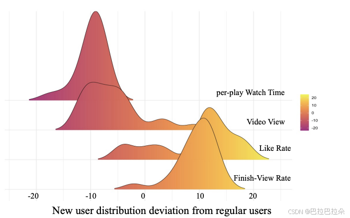
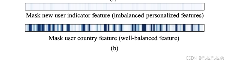
新用户与正常用户在vv、时长、点赞、完播等各个维度差异非常明显，如果将正常用户的各维度值设为原点，可以看到新用户的巨大差异。

怎么验证加一个“是否是新用户”的特征的效果呢，对于同样一个训练好的模型，给一批用户的输入，统计靠近输出的激活层的各个神经元的输出均值，然后mask掉是否是新用户这个特征，对比mask掉用户的country属性特征，再统计两者靠近输出的激活层后的各个神经元的输出，和原来不mask的做diff，会发现对于严重不平衡的特征（是否是新用户）输出没差差异，对于相对平衡的特征差异非常明显。因为是否是新用户这个特征在样本不足5%，很容易淹没在模型中，对模型整体的参数贡献非常微弱。

POSO对每个用户群体学习个性化模型，从模型层面加强对不均衡的特征的学习。

详细方案

通过gate网络学习各个用户群体的偏好，同时gate网络的输入就是能区分用户群体的特征。
$$\hat{\mathbf{x}}=C\sum _i^N[g({\mathbf{x}}^{pc}){]}_i{f}^{(i)}(\mathbf{x})$$

其中C是修正因子，gate求和没有做归一化的约束，期望存在缩放和偏移。$\mathbf{x}\in R^{d^{in}}$,$\hat{\mathbf{x}}\in R^{d^{out}}$

如果是最简单的线性模型$f(\mathbf{x})=\mathbf{Wx}$,则变成

$$\hat{\mathbf{x}}=C\sum _i^N[g({\mathbf{x}}^{pc}){]}_i{\mathbf{W}}^{(i)}\mathbf{x}$$

$\hat{\mathbf{x}}$的第$p$维计算如下
$${\hat{\mathbf{x}}}_p=C\sum _i^N\sum _{q=1}^{d^{in}}[g({\mathbf{x}}^{pc}){]}_i{\mathbf{W}}_{p,q}^{(i)}{\mathbf{x}}_q$$

这里简化处理下，让$N=d^{out},{\mathbf{W}}_{p,q}^{(i)}={\mathbf{W}}_{p,q}\forall p,qwheni=p,and{\mathbf{W}}_{p,q}\equiv 0foranyi\ne p$
变成了
$${\hat{\mathbf{x}}}_p=C\times [g({\mathbf{x}}^{pc}){]}_p\sum _{q=1}^{d^{in}}{\mathbf{W}}_{p,q}{\mathbf{x}}_q$$
等价就是
$$\hat{\mathbf{x}}=C\times [g({\mathbf{x}}^{pc})]\odot \mathbf{Wx}$$
那就是gate网络的结果和线性输出的结果直接元素级点乘

对于MLP来讲，也是如此
$$\hat{\mathbf{x}}=C\times [g({\mathbf{x}}^{pc})]\odot \sigma (\mathbf{Wx})$$

对于MMoE来讲
$$\hat{\mathbf{x}}=C\sum _i^N[g({\mathbf{x}}^{pc}){]}_i(\sum _j^{N_{expert}}[g^{task}(\mathbf{x}){]}_j{e}^{(j)}(\mathbf{x}))$$

$$\hat{\mathbf{x}}=C\sum _i^N[g({\mathbf{x}}^{pc}){]}_i[g^{task}(\mathbf{x}){]}_i{e}^{(i)}(\mathbf{x})$$

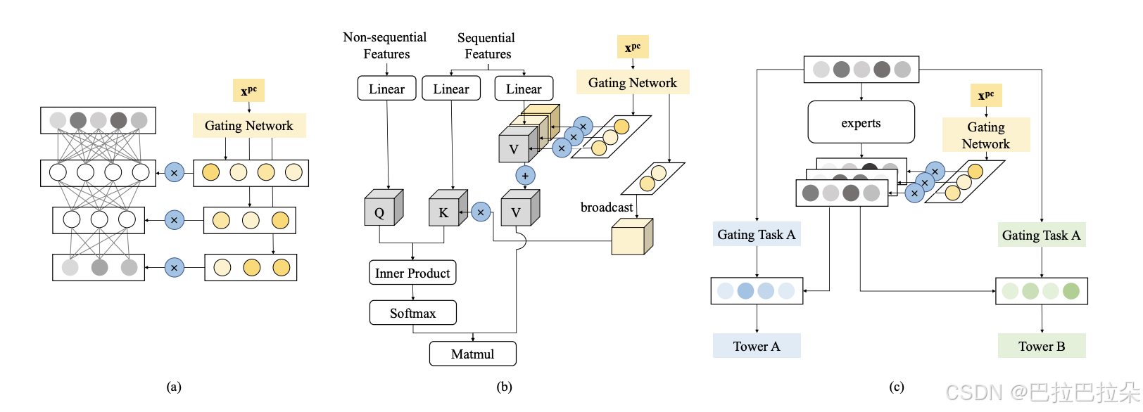
POSO接入MLP、Multi-Head Attention、MMoE的结构如下图