


📜 数据预处理系列:特征工程介绍_异常值、缺失值、编码、特征提取
什么是特征工程
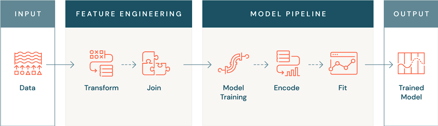
特征工程是将数据进行转换和丰富,以提高使用该数据训练模型的机器学习算法的性能的过程。
特征工程包括诸如缩放或标准化数据、对非数值数据(如文本或图像)进行编码、按时间或实体聚合数据、合并来自不同来源的数据,甚至从其他模型中转移知识等步骤。这些转换的目标是增加机器学习算法从数据集中学习的能力,从而进行更准确的预测。
为什么特征工程很重要?
特征工程之所以重要有几个原因。首先,正如前面提到的,机器学习模型有时无法处理原始数据,因此必须将数据转换为模型能够理解的数值形式。这可能涉及将文本或图像数据转换为数值形式,或创建聚合特征,例如客户的平均交易值。
有时,机器学习问题的相关特征可能存在于多个数据源中,因此有效的特征工程涉及将这些数据源连接在一起,创建一个可用的数据集。这使您可以使用所有可用的数据来训练模型,从而提高其准确性和性能。
另一个常见的情况是,其他模型的输出和学习有时可以以特征的形式重复使用于新问题,这个过程被称为迁移学习。这使您可以利用从先前模型中获得的知识来提高新模型的性能。在处理大型复杂数据集且从头开始训练模型不切实际的情况下,迁移学习特别有用。
有效的特征工程还可以在推理时生成可靠的特征,即在模型用于对新数据进行预测时。这很重要,因为推理时使用的特征必须与训练时使用的特征相同,以避免“在线/离线偏差”,即在预测时使用的特征与训练时计算的特征不同。
特征工程与其他数据转换有何不同?
特征工程的目标是创建一个可以用于构建机器学习模型的数据集。许多用于数据转换的工具和技术也被用于特征工程。
由于特征工程的重点是开发模型,因此存在一些其他特征转换所没有的要求。例如,您可能希望在组织中的多个模型或团队之间重用特征。这需要一种强大的方法来发现特征。
此外,一旦特征被重用,您将需要一种跟踪特征计算位置和方式的方法。这被称为特征血统。对于机器学习来说,可重现的特征计算尤为重要,因为特征不仅必须在训练模型时计算,而且在模型用于推断时必须以完全相同的方式重新计算。
有效的特征工程有哪些好处?
拥有有效的特征工程流水线意味着更强大的建模流程,最终得到更可靠和高性能的模型。改进用于训练和推断的特征可以对模型质量产生令人难以置信的影响,因此更好的特征意味着更好的模型。
从另一个角度来看,有效的特征工程还鼓励重用,不仅节省从业者的时间,还提高了他们模型的质量。特征重用之所以重要有两个原因:它节省时间,并且具有强大定义的特征有助于防止模型在训练和推断之间使用不同的特征数据,这通常会导致“在线/离线”偏差。
内容
☠️Outliers☠️
什么是异常值?
在数据分析中,异常值是数据集中与其他值差异很大的值,它们要么比其他值大得多,要么显著较小。异常值可能表示测量中的变异性、实验误差或新奇性。
举个现实世界的例子,长颈鹿的平均身高约为16英尺。然而,最近发现了两只身高分别为9英尺和8.5英尺的长颈鹿。与一般的长颈鹿种群相比,这两只长颈鹿被视为异常值。
在进行数据分析过程中,异常值可能会对所得结果产生异常。这意味着它们需要特别关注,并且在某些情况下需要被移除以便有效地分析数据。
-
给予异常值特别关注是数据分析过程中必要的一个方面,原因有两个:
- 异常值可能对分析结果产生负面影响。
- 异常值或其行为可能是数据分析师从分析中所需的信息。
异常值的类型
-
有两种类型的异常值:
- 单变量异常值是与单个变量相关的极端值。例如,苏丹·科森目前是世界上最高的人,身高为8英尺2.8英寸(251厘米)。这种情况被认为是单变量异常值,因为它是一个单一因素(身高)的极端情况。
- 多变量异常值是至少两个变量的异常或极端值的组合。例如,如果你正在观察一组成年人的身高和体重,你可能会观察到数据集中有一个人的身高是5英尺9英寸,这个测量值在这个特定变量的正常范围内。你可能还观察到这个人体重为110磅。同样,这个观察结果单独来看在体重这个变量的正常范围内。然而,当你将这两个观察结果结合起来考虑时,你就有了一个身高为5英尺9英寸,体重为110磅的成年人,这是一个令人惊讶的组合。这就是一个多变量异常值。
-
除了单变量和多变量异常值之间的区别,你还会看到异常值被归类为以下任何一种:
- 全局异常值(也称为点异常值)是远离数据分布的单个数据点。
- 上下文异常值(也称为条件异常值)是与同一上下文中的其他数据点显著偏离的值,这意味着如果在不同的上下文中发生,相同的值可能不被视为异常值。这类异常值通常在时间序列数据中发现。
- 集体异常值被视为与整个数据集完全不同的数据点的子集。
✨Detecting Outliers✨
import numpy as np
import pandas as pd
import seaborn as sns
from matplotlib import pyplot as plt

# !pip install missingno
import missingno as msno

from datetime import date

from sklearn.metrics import accuracy_score
from sklearn.model_selection import train_test_split
from sklearn.neighbors import LocalOutlierFactor
from sklearn.preprocessing import MinMaxScaler, LabelEncoder, StandardScaler, RobustScaler

import warnings
warnings.filterwarnings("ignore")

# pd.set_option('display.max_columns', None)
# pd.set_option('display.max_rows', None)
# pd.set_option('display.float_format', lambda x: '%.3f' % x)
# pd.set_option('display.width', 500)

!wget https://raw.githubusercontent.com/h4pZ/rose-pine-matplotlib/main/themes/rose-pine-dawn.mplstyle -P /tmp
plt.style.use("/tmp/rose-pine-dawn.mplstyle")
--2023-11-13 12:42:43--  https://raw.githubusercontent.com/h4pZ/rose-pine-matplotlib/main/themes/rose-pine-dawn.mplstyle
Resolving raw.githubusercontent.com (raw.githubusercontent.com)... 185.199.111.133, 185.199.109.133, 185.199.110.133, ...
Connecting to raw.githubusercontent.com (raw.githubusercontent.com)|185.199.111.133|:443... connected.
HTTP request sent, awaiting response... 200 OK
Length: 40905 (40K) [text/plain]
Saving to: ‘/tmp/rose-pine-dawn.mplstyle’

rose-pine-dawn.mpls 100%[===================>]  39.95K  --.-KB/s    in 0.04s

2023-11-13 12:42:44 (1.02 MB/s) - ‘/tmp/rose-pine-dawn.mplstyle’ saved [40905/40905]
home_credit = pd.read_csv("/kaggle/input/home-credit-default-risk/application_train.csv")
titanic_ = pd.read_csv("/kaggle/input/titanic/train.csv")
titanic = titanic_.copy()
titanic.describe([0.01,0.99]).T
| count | mean | std | min | 1% | 50% | 99% | max | |
|---|---|---|---|---|---|---|---|---|
| PassengerId | 891.0 | 446.000000 | 257.353842 | 1.00 | 9.9 | 446.0000 | 882.10000 | 891.0000 |
| Survived | 891.0 | 0.383838 | 0.486592 | 0.00 | 0.0 | 0.0000 | 1.00000 | 1.0000 |
| Pclass | 891.0 | 2.308642 | 0.836071 | 1.00 | 1.0 | 3.0000 | 3.00000 | 3.0000 |
| Age | 714.0 | 29.699118 | 14.526497 | 0.42 | 1.0 | 28.0000 | 65.87000 | 80.0000 |
| SibSp | 891.0 | 0.523008 | 1.102743 | 0.00 | 0.0 | 0.0000 | 5.00000 | 8.0000 |
| Parch | 891.0 | 0.381594 | 0.806057 | 0.00 | 0.0 | 0.0000 | 4.00000 | 6.0000 |
| Fare | 891.0 | 32.204208 | 49.693429 | 0.00 | 0.0 | 14.4542 | 249.00622 | 512.3292 |
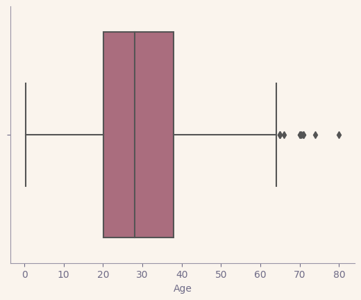
# A boxplot provides distribution information for a numerical variable. Another method could be a Histogram plot.

sns.boxplot(x = titanic["Age"])
plt.show()
q1 = titanic["Age"].quantile(0.25)
q3 = titanic["Age"].quantile(0.75)
IQR = q3 - q1
up = q3 + 1.5 * IQR
low = q1 - 1.5 * IQR
# If we want to obtain outliers, what should we do?;

titanic[(titanic["Age"] < low) | (titanic["Age"] > up)]
| PassengerId | Survived | Pclass | Name | Sex | Age | SibSp | Parch | Ticket | Fare | Cabin | Embarked | |
|---|---|---|---|---|---|---|---|---|---|---|---|---|
| 33 | 34 | 0 | 2 | Wheadon, Mr. Edward H | male | 66.0 | 0 | 0 | C.A. 24579 | 10.5000 | NaN | S |
| 54 | 55 | 0 | 1 | Ostby, Mr. Engelhart Cornelius | male | 65.0 | 0 | 1 | 113509 | 61.9792 | B30 | C |
| 96 | 97 | 0 | 1 | Goldschmidt, Mr. George B | male | 71.0 | 0 | 0 | PC 17754 | 34.6542 | A5 | C |
| 116 | 117 | 0 | 3 | Connors, Mr. Patrick | male | 70.5 | 0 | 0 | 370369 | 7.7500 | NaN | Q |
| 280 | 281 | 0 | 3 | Duane, Mr. Frank | male | 65.0 | 0 | 0 | 336439 | 7.7500 | NaN | Q |
| 456 | 457 | 0 | 1 | Millet, Mr. Francis Davis | male | 65.0 | 0 | 0 | 13509 | 26.5500 | E38 | S |
| 493 | 494 | 0 | 1 | Artagaveytia, Mr. Ramon | male | 71.0 | 0 | 0 | PC 17609 | 49.5042 | NaN | C |
| 630 | 631 | 1 | 1 | Barkworth, Mr. Algernon Henry Wilson | male | 80.0 | 0 | 0 | 27042 | 30.0000 | A23 | S |
| 672 | 673 | 0 | 2 | Mitchell, Mr. Henry Michael | male | 70.0 | 0 | 0 | C.A. 24580 | 10.5000 | NaN | S |
| 745 | 746 | 0 | 1 | Crosby, Capt. Edward Gifford | male | 70.0 | 1 | 1 | WE/P 5735 | 71.0000 | B22 | S |
| 851 | 852 | 0 | 3 | Svensson, Mr. Johan | male | 74.0 | 0 | 0 | 347060 | 7.7750 | NaN | S |
# We obtained the index information of rows containing outliers;

titanic[(titanic["Age"] < low) | (titanic["Age"] > up)].index
Index([33, 54, 96, 116, 280, 456, 493, 630, 672, 745, 851], dtype='int64')
titanic[(titanic["Age"] < low) | (titanic["Age"] > up)].any(axis=None)
True
titanic[(titanic["Age"] < low)].any(axis=None)
False
#计算df每列上下分位数界限
def outlier_thresholds(dataframe, col_name, q1=0.05, q3=0.95):

    quartile1 = dataframe[col_name].quantile(q1)
    quartile3 = dataframe[col_name].quantile(q3)
    IQR = quartile3 - quartile1
    up_limit = quartile3 + 1.5 * IQR
    low_limit = quartile1 - 1.5 * IQR

    return low_limit, up_limit
#检测df每列是否有异常值
def check_outlier(dataframe, col_name):

    low_limit, up_limit = outlier_thresholds(dataframe, col_name)

    if dataframe[(dataframe[col_name] > up_limit) | (dataframe[col_name] < low_limit)].any(axis=None):

        return True

    else:

        return False
check_outlier(titanic, "Age")
False
def grab_col_names(dataframe, cat_th=10, car_th=20):

    """
    返回数据集中的分类、数值和分类但基数变量的名称。
    注意:看起来像数值的分类变量也包括在分类变量中。

    Parameters
    ------
        dataframe: dataframe
                The dataframe for which variable names are to be obtained.
        cat_th: int, optional
                Class threshold value for numerical but categorical variables.
        car_th: int, optional
                Class threshold value for categorical but cardinal variables.

    Returns
    ------
        cat_cols: list
                List of categorical variables.
        num_cols: list
                List of numerical variables.
        cat_but_car: list
                List of categorical but cardinal variables.

    Examples
    ------
        import seaborn as sns
        df = sns.load_dataset("iris")
        print(grab_col_names(df))


    Notes
    ------
        cat_cols + num_cols + cat_but_car = total number of variables
        num_but_cat is within cat_cols.
        The sum of the 3 lists returned is equal to the total number of variables: cat_cols + num_cols + cat_but_car = number of variables

    """

    # cat_cols, cat_but_car

    cat_cols = [col for col in dataframe.columns if dataframe[col].dtypes == "O"]
    num_but_cat = [col for col in dataframe.columns if dataframe[col].nunique() < cat_th and
                   dataframe[col].dtypes != "O"]
    cat_but_car = [col for col in dataframe.columns if dataframe[col].nunique() > car_th and
                   dataframe[col].dtypes == "O"]
    cat_cols = cat_cols + num_but_cat
    cat_cols = [col for col in cat_cols if col not in cat_but_car]

    # num_cols

    num_cols = [col for col in dataframe.columns if dataframe[col].dtypes != "O"]
    num_cols = [col for col in num_cols if col not in num_but_cat]

    print(f"Observations: {dataframe.shape[0]}")
    print(f"Variables: {dataframe.shape[1]}")
    print(f'cat_cols: {len(cat_cols)}')
    print(f'num_cols: {len(num_cols)}')
    print(f'cat_but_car: {len(cat_but_car)}')
    print(f'num_but_cat: {len(num_but_cat)}')

    return cat_cols, num_cols, cat_but_car
cat_cols, num_cols, cat_but_car = grab_col_names(titanic)
Observations: 891
Variables: 12
cat_cols: 6
num_cols: 3
cat_but_car: 3
num_but_cat: 4
🗨️ Comment:
- The number of num_but_cat is already included within the cat_cols, representing only the quantity identified.
num_cols = [col for col in num_cols if col not in "PassengerId"]
num_cols
['Age', 'Fare']
🗨️ Comment:
- We need to distinguish ID or date variables since they can also be considered as numerical.
for col in num_cols:

    print(col, check_outlier(titanic, col))
Age False
Fare True
#检测df每列上下边界
def outliner_detecter(df,cols):

    temp = pd.DataFrame()

    for col in cols:

        q1 = df[col].quantile(0.05)
        q3 = df[col].quantile(0.95)
        IQR = q3 - q1
        up = q3 + 1.5 * IQR
        low = q1 - 1.5 * IQR
        temp.loc[col, "Min"] = df[col].min()
        temp.loc[col, "Low_Limit"] = low
        temp.loc[col,"Up_Limit"] = up
        temp.loc[col, "Max"] = df[col].max()

    return print(temp.astype(int).to_markdown())
outliner_detecter(titanic,num_cols)
|      |   Min |   Low_Limit |   Up_Limit |   Max |
|:-----|------:|------------:|-----------:|------:|
| Age  |     0 |         -74 |        134 |    80 |
| Fare |     0 |        -150 |        269 |   512 |
📄 Notes:
- outlier_thresholds: 使用此函数,我们可以显示下限和上限。
- check_outlier: 此函数可用于检查变量是否包含异常值。
- grab_col_names: 使用此函数,我们可以识别数值、分类、数值型分类或无信息分类变量。参数可能因数据集而异。
- outlier_detector: 在此函数中,我们不仅可以查看下限和上限,还可以查看最小值和最大值。如果需要,还可以包括其他统计信息,如中位数。
✨Accessing Outliers✨
# 获取df指定列的异常值
def grab_outliers(dataframe, col_name, index=False):

    low, up = outlier_thresholds(dataframe, col_name)

    outliers = dataframe[(dataframe[col_name] < low) | (dataframe[col_name] > up)]

    if len(outliers) > 10:
        print(outliers.head())

    else:
        print(outliers)

    if index:
        outlier_index = outliers.index

        return outlier_index
grab_outliers(titanic, "Fare")
     PassengerId  Survived  Pclass                                Name  \
258          259         1       1                    Ward, Miss. Anna
679          680         1       1  Cardeza, Mr. Thomas Drake Martinez
737          738         1       1              Lesurer, Mr. Gustave J

        Sex   Age  SibSp  Parch    Ticket      Fare        Cabin Embarked
258  female  35.0      0      0  PC 17755  512.3292          NaN        C
679    male  36.0      0      1  PC 17755  512.3292  B51 B53 B55        C
737    male  35.0      0      0  PC 17755  512.3292         B101        C
age_indexes = grab_outliers(titanic, "Fare", True)
     PassengerId  Survived  Pclass                                Name  \
258          259         1       1                    Ward, Miss. Anna
679          680         1       1  Cardeza, Mr. Thomas Drake Martinez
737          738         1       1              Lesurer, Mr. Gustave J

        Sex   Age  SibSp  Parch    Ticket      Fare        Cabin Embarked
258  female  35.0      0      0  PC 17755  512.3292          NaN        C
679    male  36.0      0      1  PC 17755  512.3292  B51 B53 B55        C
737    male  35.0      0      0  PC 17755  512.3292         B101        C
age_indexes
Index([258, 679, 737], dtype='int64')
🗨️ Comment:
- 如果检测到超过10个异常值,则打印前5行。
- 如果想要访问索引信息,可以将参数 “index=False” 设置为 True。
✨Removing Outliers✨
titanic.shape
(891, 12)
#移除异常值
def remove_outlier(dataframe, col_name):

    low_limit, up_limit = outlier_thresholds(dataframe, col_name)
    df_without_outliers = dataframe[~((dataframe[col_name] < low_limit) | (dataframe[col_name] > up_limit))]

    return df_without_outliers
for col in num_cols:

    new_df = remove_outlier(titanic, col)
titanic.shape[0] - new_df.shape[0]
3
titanic.describe([0.01,0.99]).T
| count | mean | std | min | 1% | 50% | 99% | max | |
|---|---|---|---|---|---|---|---|---|
| PassengerId | 891.0 | 446.000000 | 257.353842 | 1.00 | 9.9 | 446.0000 | 882.10000 | 891.0000 |
| Survived | 891.0 | 0.383838 | 0.486592 | 0.00 | 0.0 | 0.0000 | 1.00000 | 1.0000 |
| Pclass | 891.0 | 2.308642 | 0.836071 | 1.00 | 1.0 | 3.0000 | 3.00000 | 3.0000 |
| Age | 714.0 | 29.699118 | 14.526497 | 0.42 | 1.0 | 28.0000 | 65.87000 | 80.0000 |
| SibSp | 891.0 | 0.523008 | 1.102743 | 0.00 | 0.0 | 0.0000 | 5.00000 | 8.0000 |
| Parch | 891.0 | 0.381594 | 0.806057 | 0.00 | 0.0 | 0.0000 | 4.00000 | 6.0000 |
| Fare | 891.0 | 32.204208 | 49.693429 | 0.00 | 0.0 | 14.4542 | 249.00622 | 512.3292 |
🗨️ Comment:
当我们在一个单元格中删除异常值时,其他变量中的数据也会受到影响。因此,有时候采用截断处理而不是删除可能更合适。
✨Re-Assignment with Thresholds✨
titanic = titanic_.copy()
titanic.shape
(891, 12)
for col in num_cols:

    print(col, check_outlier(titanic, col))
Age False
Fare True
#替换超过上下文边界的值为边界值
def corr_skew_outliner(df, cols):

    for col in cols:

        Q1 = df[col].quantile(0.05)
        Q3 = df[col].quantile(0.95)
        df.loc[df[col] < Q1, col] = Q1
        df.loc[df[col] > Q3, col] = Q3
        #df[col] = np.sqrt(df[col])

    return df
corr_skew_outliner(titanic, num_cols).head()
| PassengerId | Survived | Pclass | Name | Sex | Age | SibSp | Parch | Ticket | Fare | Cabin | Embarked | |
|---|---|---|---|---|---|---|---|---|---|---|---|---|
| 0 | 1 | 0 | 3 | Braund, Mr. Owen Harris | male | 22.0 | 1 | 0 | A/5 21171 | 7.2500 | NaN | S |
| 1 | 2 | 1 | 1 | Cumings, Mrs. John Bradley (Florence Briggs Th... | female | 38.0 | 1 | 0 | PC 17599 | 71.2833 | C85 | C |
| 2 | 3 | 1 | 3 | Heikkinen, Miss. Laina | female | 26.0 | 0 | 0 | STON/O2. 3101282 | 7.9250 | NaN | S |
| 3 | 4 | 1 | 1 | Futrelle, Mrs. Jacques Heath (Lily May Peel) | female | 35.0 | 1 | 0 | 113803 | 53.1000 | C123 | S |
| 4 | 5 | 0 | 3 | Allen, Mr. William Henry | male | 35.0 | 0 | 0 | 373450 | 8.0500 | NaN | S |
titanic.describe([0.01,0.99]).T
| count | mean | std | min | 1% | 50% | 99% | max | |
|---|---|---|---|---|---|---|---|---|
| PassengerId | 891.0 | 446.000000 | 257.353842 | 1.000 | 9.900 | 446.0000 | 882.10000 | 891.00000 |
| Survived | 891.0 | 0.383838 | 0.486592 | 0.000 | 0.000 | 0.0000 | 1.00000 | 1.00000 |
| Pclass | 891.0 | 2.308642 | 0.836071 | 1.000 | 1.000 | 3.0000 | 3.00000 | 3.00000 |
| Age | 714.0 | 29.440476 | 13.523898 | 4.000 | 4.000 | 28.0000 | 56.00000 | 56.00000 |
| SibSp | 891.0 | 0.523008 | 1.102743 | 0.000 | 0.000 | 0.0000 | 5.00000 | 8.00000 |
| Parch | 891.0 | 0.381594 | 0.806057 | 0.000 | 0.000 | 0.0000 | 4.00000 | 6.00000 |
| Fare | 891.0 | 27.857570 | 29.112872 | 7.225 | 7.225 | 14.4542 | 112.07915 | 112.07915 |
titanic.shape
(891, 12)
🗨️ Comment:
- 如上所述,这次我们使用了截断方法来保留所有数据,而不是丢失数据。然而,删除或截断方法的选择可能因数据集而异。这完全是基于解释的偏好过程。
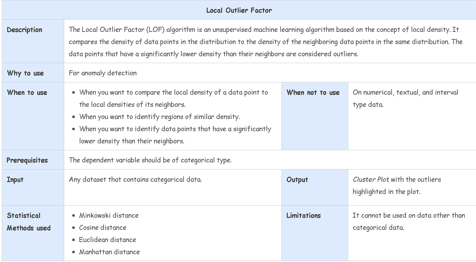
✨局部离群因子(Local Outlier Factor)✨
局部离群因子(Local Outlier Factor)根据数据点在分布中与其邻居的密度关系来检测离群值或偏差。它识别数据集中的局部离群值,这些离群值在数据集的其他区域中并不是离群值。
例如,考虑一个数据集中非常密集的数据点簇。其中一个数据点与密集簇的距离很近。这个数据点被认为是一个离群值。在同一个数据集中,一个稀疏簇中的数据点可能看起来是一个离群值,但实际上与其邻居的距离相似。
一个正常的数据点的局部离群因子(LOF)在1到1.5之间,而离群值的LOF要高得多。如果一个数据点的LOF为10,这意味着其邻居的平均密度比数据点的局部密度高十倍。
局部离群因子方法用于检测地理数据、视频流或网络入侵检测中的离群值。
-
通过以下方式确定数据点的LOF分数:
- 邻居数量
- 用于构建数据结构的树算法
- 叶子大小以定义树算法的深度
- 度量函数以定义两个点之间的距离
- 超参数调整
- 维度降低和方差
一个例子:它允许我们通过对观测值在其相应位置的密度进行评分来定义离群值。密度是该观测单元与其邻居的语义相似性。例如,仅仅年龄为17岁可能不会被视为离群值。然而,年龄为17岁且已经结过3次婚可能不太正常。我们可以将其视为离群值。
df = sns.load_dataset('diamonds')
df = df.select_dtypes(include=['float64', 'int64'])
df.isnull().sum() # seems there is not any NaN value.
carat    0
depth    0
table    0
price    0
x        0
y        0
z        0
dtype: int64
df.head()
| carat | depth | table | price | x | y | z | |
|---|---|---|---|---|---|---|---|
| 0 | 0.23 | 61.5 | 55.0 | 326 | 3.95 | 3.98 | 2.43 |
| 1 | 0.21 | 59.8 | 61.0 | 326 | 3.89 | 3.84 | 2.31 |
| 2 | 0.23 | 56.9 | 65.0 | 327 | 4.05 | 4.07 | 2.31 |
| 3 | 0.29 | 62.4 | 58.0 | 334 | 4.20 | 4.23 | 2.63 |
| 4 | 0.31 | 63.3 | 58.0 | 335 | 4.34 | 4.35 | 2.75 |
df.shape
(53940, 7)
for col in df.columns:

    print(col, check_outlier(df, col))
carat True
depth True
table True
price False
x False
y True
z True
clf = LocalOutlierFactor(n_neighbors=20)
clf.fit_predict(df)
array([-1, -1, -1, ..., 1, 1, 1])
# Local Outlier Factor Scores

df_scores = clf.negative_outlier_factor_
df_scores[0:5]
# df_scores = -df_scores (If we want to keep positive values)
array([-1.58352526, -1.59732899, -1.62278873, -1.33002541, -1.30712521])
scores = pd.DataFrame(np.sort(df_scores))
scores.plot(stacked=True, xlim=[0, 50], style='.-')
plt.show()
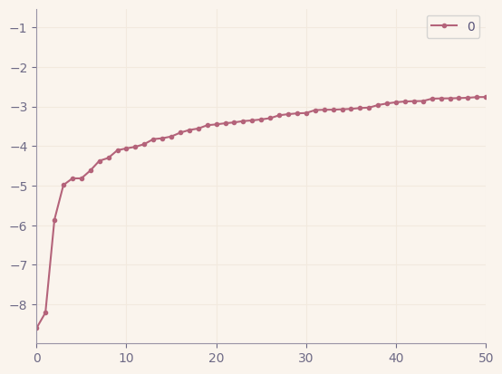
🗨️ Comment:
- LOF分数越接近-10,越糟糕。然而,我们需要设定一个阈值。
- 如我们所见,在第三个点之后,斜率发生了显著变化。
th = np.sort(df_scores)[3]
th
-4.984151747711709
🗨️ Comment:
- LOF分数越接近-10,越糟糕。然而,我们需要设定一个阈值。
- 如我们所见,在第三个点之后,斜率发生了显著变化。
- 我们已将此值设定为阈值。我们将考虑那些小于此值的点为异常值。
df[df_scores < th]
| carat | depth | table | price | x | y | z | |
|---|---|---|---|---|---|---|---|
| 41918 | 1.03 | 78.2 | 54.0 | 1262 | 5.72 | 5.59 | 4.42 |
| 48410 | 0.51 | 61.8 | 54.7 | 1970 | 5.12 | 5.15 | 31.80 |
| 49189 | 0.51 | 61.8 | 55.0 | 2075 | 5.15 | 31.80 | 5.12 |
df[df_scores < th].shape
(3, 7)
df.describe([0.01, 0.05, 0.75, 0.90, 0.99]).T
| count | mean | std | min | 1% | 5% | 50% | 75% | 90% | 99% | max | |
|---|---|---|---|---|---|---|---|---|---|---|---|
| carat | 53940.0 | 0.797940 | 0.474011 | 0.2 | 0.24 | 0.30 | 0.70 | 1.04 | 1.51 | 2.18 | 5.01 |
| depth | 53940.0 | 61.749405 | 1.432621 | 43.0 | 57.90 | 59.30 | 61.80 | 62.50 | 63.30 | 65.60 | 79.00 |
| table | 53940.0 | 57.457184 | 2.234491 | 43.0 | 53.00 | 54.00 | 57.00 | 59.00 | 60.00 | 64.00 | 95.00 |
| price | 53940.0 | 3932.799722 | 3989.439738 | 326.0 | 429.00 | 544.00 | 2401.00 | 5324.25 | 9821.00 | 17378.22 | 18823.00 |
| x | 53940.0 | 5.731157 | 1.121761 | 0.0 | 4.02 | 4.29 | 5.70 | 6.54 | 7.31 | 8.36 | 10.74 |
| y | 53940.0 | 5.734526 | 1.142135 | 0.0 | 4.04 | 4.30 | 5.71 | 6.54 | 7.30 | 8.34 | 58.90 |
| z | 53940.0 | 3.538734 | 0.705699 | 0.0 | 2.48 | 2.65 | 3.53 | 4.04 | 4.52 | 5.15 | 31.80 |
🗨️ Comment:
为什么将这三个观测值视为异常值?让我们来检查一下。- 第一个显而易见的细节是观测编号为"41918"的观测值具有"depth"值为"78.200"。在我们的主数据集中,“depth"变量的最大值显示为"79.000”。但为什么它没有选择最高值,而是选择了低于最大值的值?这只是一种推断。因为这里存在多变量效应,当深度值为当前值时,可能与其他变量的交互存在不一致。让我们继续检查。
- 观测编号为"48410"的观测值具有"z"值为"31.800"。同时,这个z值对应于最大值。当然,这种情况也属于与其他变量相关的异常值,就像前一个情况一样。可以推断出当一个变量取值时,它与另一个变量的值不一致。
df[df_scores < th].index
Index([41918, 48410, 49189], dtype='int64')
df[df_scores < th].drop(axis=0, labels=df[df_scores < th].index)
| carat | depth | table | price | x | y | z |
|---|
🗨️ Comment:
- 如果我们对树方法感兴趣,在这一点上,我们应该尽量不去触碰异常值去除和截断方法,至少在最基本的层面上是如此。然而,如果需要进行一些调整,可以进行非常小的调整(0.01 - 0.99)。
- 如果更喜欢线性方法;如果异常值的数量较少,可能更倾向于删除;或者可以将截断作为单变量方法来进行。
def take_a_look(df):

    print(pd.DataFrame({'Rows': [df.shape[0]], 'Columns': [df.shape[1]]}, index=["Shape"]).to_markdown())
    print("\n")
    print(pd.DataFrame(df.dtypes, columns=["Type"]).to_markdown())
    print("\n")
    print(df.head().to_markdown(index=False))
    print("\n")
    print(df.isnull().sum().to_markdown())
    print("\n")
    print(df.describe([0.01, 0.25, 0.75, 0.99]).astype(int).T.to_markdown())
take_a_look(df)
|       |   Rows |   Columns |
|:------|-------:|----------:|
| Shape |  53940 |         7 |


|       | Type    |
|:------|:--------|
| carat | float64 |
| depth | float64 |
| table | float64 |
| price | int64   |
| x     | float64 |
| y     | float64 |
| z     | float64 |


|   carat |   depth |   table |   price |    x |    y |    z |
|--------:|--------:|--------:|--------:|-----:|-----:|-----:|
|    0.23 |    61.5 |      55 |     326 | 3.95 | 3.98 | 2.43 |
|    0.21 |    59.8 |      61 |     326 | 3.89 | 3.84 | 2.31 |
|    0.23 |    56.9 |      65 |     327 | 4.05 | 4.07 | 2.31 |
|    0.29 |    62.4 |      58 |     334 | 4.2  | 4.23 | 2.63 |
|    0.31 |    63.3 |      58 |     335 | 4.34 | 4.35 | 2.75 |


|       |   0 |
|:------|----:|
| carat |   0 |
| depth |   0 |
| table |   0 |
| price |   0 |
| x     |   0 |
| y     |   0 |
| z     |   0 |


|       |   count |   mean |   std |   min |   1% |   25% |   50% |   75% |   99% |   max |
|:------|--------:|-------:|------:|------:|-----:|------:|------:|------:|------:|------:|
| carat |   53940 |      0 |     0 |     0 |    0 |     0 |     0 |     1 |     2 |     5 |
| depth |   53940 |     61 |     1 |    43 |   57 |    61 |    61 |    62 |    65 |    79 |
| table |   53940 |     57 |     2 |    43 |   53 |    56 |    57 |    59 |    64 |    95 |
| price |   53940 |   3932 |  3989 |   326 |  429 |   950 |  2401 |  5324 | 17378 | 18823 |
| x     |   53940 |      5 |     1 |     0 |    4 |     4 |     5 |     6 |     8 |    10 |
| y     |   53940 |      5 |     1 |     0 |    4 |     4 |     5 |     6 |     8 |    58 |
| z     |   53940 |      3 |     0 |     0 |    2 |     2 |     3 |     4 |     5 |    31 |
🤔缺失值 🤔
什么是缺失值?
缺失值是指数据集中一个或多个变量具有缺失或未定义(NULL)值的情况。这些缺失值可能是由于数据收集或数据录入过程中的错误导致的。缺失值可能对数据分析和机器学习模型造成重大问题,因为它们可能导致错误的结果或误导性的分析。处理缺失值是数据科学和统计学中至关重要的方面。
缺失数据的类型:
-
完全随机缺失 Missing Completely At Random(MCAR):在这种类型的缺失中,缺失值是随机的,与其他变量无关。例如,忘记填写调查的某个部分就是这种类型的例子。
-
随机缺失 Missing At Random(MAR):这种类型的缺失意味着缺失值与其他观察到的变量有关,但还有其他可用的变量可以用来预测缺失值的水平。例如,如果年龄数据缺失,但性别数据可用,可能可以使用年龄和性别之间的关系来预测年龄。
-
非随机缺失 Missing Not At Random(MNAR):这种类型的缺失表明缺失值与其他变量有关,并且没有其他可用的变量来预测缺失值的水平。MNAR是最具挑战性的缺失数据类型,通常需要更深入地了解缺失数据的原因。
处理缺失数据:
可以使用几种不同的方法来处理缺失数据:
-
删除缺失值:这涉及从数据集中删除具有缺失数据的观察。然而,这种方法可能会导致重要信息的丢失,如果数据集很小,则不应使用此方法。
-
填补缺失值:可以使用各种方法对缺失值进行填补。可以使用统计值(如中位数、平均值、众数)进行填补,也可以使用机器学习模型来预测缺失值。
-
对缺失值进行分类:可以根据缺失情况将缺失数据视为一个单独的类别。这可以是一种有用的方法,以防止数据丢失。
缺失数据对建模的影响:
缺失数据可能会影响模型的结果和预测。具有缺失数据的观察结果可能导致误导性的结果。此外,缺失数据的处理也可能影响模型的性能。因此,处理缺失数据对模型准确性有重大影响。
✨检测缺失值 ✨
# 检测是否有缺失值

titanic.isnull().values.any()
True
# 统计缺失值

titanic.isnull().sum()
PassengerId      0
Survived         0
Pclass           0
Name             0
Sex              0
Age            177
SibSp            0
Parch            0
Ticket           0
Fare             0
Cabin          687
Embarked         2
dtype: int64
# 统计非缺失值

titanic.notnull().sum()
PassengerId    891
Survived       891
Pclass         891
Name           891
Sex            891
Age            714
SibSp          891
Parch          891
Ticket         891
Fare           891
Cabin          204
Embarked       889
dtype: int64
# 统计缺失值数量

titanic.isnull().sum().sum()
866
# 查看每列中至少一个缺失值

titanic[titanic.isnull().any(axis=1)].head()
| PassengerId | Survived | Pclass | Name | Sex | Age | SibSp | Parch | Ticket | Fare | Cabin | Embarked | |
|---|---|---|---|---|---|---|---|---|---|---|---|---|
| 0 | 1 | 0 | 3 | Braund, Mr. Owen Harris | male | 22.0 | 1 | 0 | A/5 21171 | 7.2500 | NaN | S |
| 2 | 3 | 1 | 3 | Heikkinen, Miss. Laina | female | 26.0 | 0 | 0 | STON/O2. 3101282 | 7.9250 | NaN | S |
| 4 | 5 | 0 | 3 | Allen, Mr. William Henry | male | 35.0 | 0 | 0 | 373450 | 8.0500 | NaN | S |
| 5 | 6 | 0 | 3 | Moran, Mr. James | male | NaN | 0 | 0 | 330877 | 8.4583 | NaN | Q |
| 7 | 8 | 0 | 3 | Palsson, Master. Gosta Leonard | male | 4.0 | 3 | 1 | 349909 | 21.0750 | NaN | S |
# 查看非缺失的完整数据

titanic[titanic.notnull().all(axis=1)].head()
| PassengerId | Survived | Pclass | Name | Sex | Age | SibSp | Parch | Ticket | Fare | Cabin | Embarked | |
|---|---|---|---|---|---|---|---|---|---|---|---|---|
| 1 | 2 | 1 | 1 | Cumings, Mrs. John Bradley (Florence Briggs Th... | female | 38.0 | 1 | 0 | PC 17599 | 71.2833 | C85 | C |
| 3 | 4 | 1 | 1 | Futrelle, Mrs. Jacques Heath (Lily May Peel) | female | 35.0 | 1 | 0 | 113803 | 53.1000 | C123 | S |
| 6 | 7 | 0 | 1 | McCarthy, Mr. Timothy J | male | 54.0 | 0 | 0 | 17463 | 51.8625 | E46 | S |
| 10 | 11 | 1 | 3 | Sandstrom, Miss. Marguerite Rut | female | 4.0 | 1 | 1 | PP 9549 | 16.7000 | G6 | S |
| 11 | 12 | 1 | 1 | Bonnell, Miss. Elizabeth | female | 56.0 | 0 | 0 | 113783 | 26.5500 | C103 | S |
def missing_values_table(dataframe, na_name=False):

    na_columns = [col for col in dataframe.columns if dataframe[col].isnull().sum() > 0]

    n_miss = dataframe[na_columns].isnull().sum().sort_values(ascending=False)
    ratio = (dataframe[na_columns].isnull().sum() / dataframe.shape[0] * 100).sort_values(ascending=False)

    missing_df = pd.concat([n_miss, np.round(ratio, 2)], axis=1, keys=['n_miss', 'ratio']).to_markdown()

    print(missing_df, end="\n")

    if na_name:

        return na_columns
missing_values_table(titanic)
|          |   n_miss |   ratio |
|:---------|---------:|--------:|
| Cabin    |      687 |   77.1  |
| Age      |      177 |   19.87 |
| Embarked |        2 |    0.22 |
✨处理缺失值 ✨
titanic.shape
(891, 12)
titanic.isnull().sum().sum()
866
titanic.dropna().shape
(183, 12)
🗨️ Comment:
- 我们可以使用
dropna方法删除具有缺失值的行。然而,正如我们所见,这可能导致数据的显著损失。
titanic = titanic_.copy()
titanic["Age"].fillna(titanic["Age"].mean()).isnull().sum()
0
titanic["Age"].fillna(titanic["Age"].median()).isnull().sum()
0
titanic["Age"].fillna(0).isnull().sum()
0
🗨️ Comment:
- 它也可以用平均值、中位数或所需的固定值来填充。
titanic = titanic_.copy()
# For numerical features;

titanic.apply(lambda x: x.fillna(x.mean()) if x.dtype != "O" else x, axis=0).head()
| PassengerId | Survived | Pclass | Name | Sex | Age | SibSp | Parch | Ticket | Fare | Cabin | Embarked | |
|---|---|---|---|---|---|---|---|---|---|---|---|---|
| 0 | 1 | 0 | 3 | Braund, Mr. Owen Harris | male | 22.0 | 1 | 0 | A/5 21171 | 7.2500 | NaN | S |
| 1 | 2 | 1 | 1 | Cumings, Mrs. John Bradley (Florence Briggs Th... | female | 38.0 | 1 | 0 | PC 17599 | 71.2833 | C85 | C |
| 2 | 3 | 1 | 3 | Heikkinen, Miss. Laina | female | 26.0 | 0 | 0 | STON/O2. 3101282 | 7.9250 | NaN | S |
| 3 | 4 | 1 | 1 | Futrelle, Mrs. Jacques Heath (Lily May Peel) | female | 35.0 | 1 | 0 | 113803 | 53.1000 | C123 | S |
| 4 | 5 | 0 | 3 | Allen, Mr. William Henry | male | 35.0 | 0 | 0 | 373450 | 8.0500 | NaN | S |
# For handling missing values in categorical variables;
# titanic["Embarked"].fillna(titanic["Embarked"].mode()[0]).isnull().sum()
# titanic["Embarked"].fillna("missing")
# You can fill the missing values with the mode of the "Embarked" variable or with the string "missing."
titanic.apply(lambda x: x.fillna(x.mode()[0]) if (x.dtype == "O" and len(x.unique()) <= 10) else x, axis=0).isnull().sum()
PassengerId      0
Survived         0
Pclass           0
Name             0
Sex              0
Age            177
SibSp            0
Parch            0
Ticket           0
Fare             0
Cabin          687
Embarked         0
dtype: int64
for col in cat_cols:
    if titanic[col].isnull().sum() > 0:
        mode_value = titanic[col].mode()[0]
        titanic[col].fillna(mode_value, inplace=True)
titanic.isnull().sum()
PassengerId      0
Survived         0
Pclass           0
Name             0
Sex              0
Age            177
SibSp            0
Parch            0
Ticket           0
Fare             0
Cabin          687
Embarked         0
dtype: int64
titanic.loc[(titanic["Age"].isnull()) & (titanic["Sex"]=="female"), "Age"] = titanic.groupby("Sex")["Age"].mean()["female"]

titanic.loc[(titanic["Age"].isnull()) & (titanic["Sex"]=="male"), "Age"] = titanic.groupby("Sex")["Age"].mean()["male"]
titanic.isnull().sum()
PassengerId      0
Survived         0
Pclass           0
Name             0
Sex              0
Age              0
SibSp            0
Parch            0
Ticket           0
Fare             0
Cabin          687
Embarked         0
dtype: int64
🗨️ Comment:
- 可以用性别的中位数值替换缺失的年龄值。
✨Predicting Missing Values with Machine Learning✨
titanic = titanic_.copy()
cat_cols, num_cols, cat_but_car = grab_col_names(titanic)
Observations: 891
Variables: 12
cat_cols: 6
num_cols: 3
cat_but_car: 3
num_but_cat: 4
print("Categorical Columns:", cat_cols)
print("Numerical Columns:", num_cols)
print("Cardinals (Categorical but not informative):", cat_but_car)
Categorical Columns: ['Sex', 'Embarked', 'Survived', 'Pclass', 'SibSp', 'Parch']
Numerical Columns: ['PassengerId', 'Age', 'Fare']
Cardinals (Categorical but not informative): ['Name', 'Ticket', 'Cabin']
num_cols = [col for col in num_cols if col not in "PassengerId"]
for_predict = pd.get_dummies(titanic[cat_cols + num_cols], drop_first=True)
for_predict.head()
| Survived | Pclass | SibSp | Parch | Age | Fare | Sex_male | Embarked_Q | Embarked_S | |
|---|---|---|---|---|---|---|---|---|---|
| 0 | 0 | 3 | 1 | 0 | 22.0 | 7.2500 | True | False | True |
| 1 | 1 | 1 | 1 | 0 | 38.0 | 71.2833 | False | False | False |
| 2 | 1 | 3 | 0 | 0 | 26.0 | 7.9250 | False | False | True |
| 3 | 1 | 1 | 1 | 0 | 35.0 | 53.1000 | False | False | True |
| 4 | 0 | 3 | 0 | 0 | 35.0 | 8.0500 | True | False | True |
scaler = MinMaxScaler()
for_predict = pd.DataFrame(scaler.fit_transform(for_predict), columns=for_predict.columns)
for_predict.head()
| Survived | Pclass | SibSp | Parch | Age | Fare | Sex_male | Embarked_Q | Embarked_S | |
|---|---|---|---|---|---|---|---|---|---|
| 0 | 0.0 | 1.0 | 0.125 | 0.0 | 0.271174 | 0.014151 | 1.0 | 0.0 | 1.0 |
| 1 | 1.0 | 0.0 | 0.125 | 0.0 | 0.472229 | 0.139136 | 0.0 | 0.0 | 0.0 |
| 2 | 1.0 | 1.0 | 0.000 | 0.0 | 0.321438 | 0.015469 | 0.0 | 0.0 | 1.0 |
| 3 | 1.0 | 0.0 | 0.125 | 0.0 | 0.434531 | 0.103644 | 0.0 | 0.0 | 1.0 |
| 4 | 0.0 | 1.0 | 0.000 | 0.0 | 0.434531 | 0.015713 | 1.0 | 0.0 | 1.0 |
🗨️ Comment:
- 我们对数据中的值应用了标准化,将其缩放在0和1之间。在使用机器学习模型之前,我们需要将数据转换为这种形式。
from sklearn.impute import KNNImputer

imputer = KNNImputer(n_neighbors=5)

for_predict = pd.DataFrame(imputer.fit_transform(for_predict), columns=for_predict.columns)
for_predict.head()
| Survived | Pclass | SibSp | Parch | Age | Fare | Sex_male | Embarked_Q | Embarked_S | |
|---|---|---|---|---|---|---|---|---|---|
| 0 | 0.0 | 1.0 | 0.125 | 0.0 | 0.271174 | 0.014151 | 1.0 | 0.0 | 1.0 |
| 1 | 1.0 | 0.0 | 0.125 | 0.0 | 0.472229 | 0.139136 | 0.0 | 0.0 | 0.0 |
| 2 | 1.0 | 1.0 | 0.000 | 0.0 | 0.321438 | 0.015469 | 0.0 | 0.0 | 1.0 |
| 3 | 1.0 | 0.0 | 0.125 | 0.0 | 0.434531 | 0.103644 | 0.0 | 0.0 | 1.0 |
| 4 | 0.0 | 1.0 | 0.000 | 0.0 | 0.434531 | 0.015713 | 1.0 | 0.0 | 1.0 |
🗨️ Comment:
- 我们可以使用机器学习模型来填充缺失值。
- KNN(K最近邻)是一种基于距离的方法,它查看一个点(值)的邻居,并预测最适合它的值。
- 通过取五个最近邻的平均值,添加一个新值。
- 到目前为止,填充缺失值的工作已经完成。然而,如果你看一下外观,它仍然保持在标准化的形式。因此,我们需要反转这个过程,将其转换回正常形式。
for_predict = pd.DataFrame(scaler.inverse_transform(for_predict), columns=for_predict.columns)
for_predict.head()
| Survived | Pclass | SibSp | Parch | Age | Fare | Sex_male | Embarked_Q | Embarked_S | |
|---|---|---|---|---|---|---|---|---|---|
| 0 | 0.0 | 3.0 | 1.0 | 0.0 | 22.0 | 7.2500 | 1.0 | 0.0 | 1.0 |
| 1 | 1.0 | 1.0 | 1.0 | 0.0 | 38.0 | 71.2833 | 0.0 | 0.0 | 0.0 |
| 2 | 1.0 | 3.0 | 0.0 | 0.0 | 26.0 | 7.9250 | 0.0 | 0.0 | 1.0 |
| 3 | 1.0 | 1.0 | 1.0 | 0.0 | 35.0 | 53.1000 | 0.0 | 0.0 | 1.0 |
| 4 | 0.0 | 3.0 | 0.0 | 0.0 | 35.0 | 8.0500 | 1.0 | 0.0 | 1.0 |
📄 Notes:
- 所以,如果你想看到分配了哪些值或观察到的变化,你可以做什么?
titanic["Age_Imputed_KNN"] = for_predict[["Age"]]
titanic.loc[titanic["Age"].isnull(), ["Age", "Age_Imputed_KNN"]].head()
| Age | Age_Imputed_KNN | |
|---|---|---|
| 5 | NaN | 47.8 |
| 17 | NaN | 37.6 |
| 19 | NaN | 12.2 |
| 26 | NaN | 32.8 |
| 28 | NaN | 17.6 |
titanic.loc[titanic["Age"].isnull()].head()
| PassengerId | Survived | Pclass | Name | Sex | Age | SibSp | Parch | Ticket | Fare | Cabin | Embarked | Age_Imputed_KNN | |
|---|---|---|---|---|---|---|---|---|---|---|---|---|---|
| 5 | 6 | 0 | 3 | Moran, Mr. James | male | NaN | 0 | 0 | 330877 | 8.4583 | NaN | Q | 47.8 |
| 17 | 18 | 1 | 2 | Williams, Mr. Charles Eugene | male | NaN | 0 | 0 | 244373 | 13.0000 | NaN | S | 37.6 |
| 19 | 20 | 1 | 3 | Masselmani, Mrs. Fatima | female | NaN | 0 | 0 | 2649 | 7.2250 | NaN | C | 12.2 |
| 26 | 27 | 0 | 3 | Emir, Mr. Farred Chehab | male | NaN | 0 | 0 | 2631 | 7.2250 | NaN | C | 32.8 |
| 28 | 29 | 1 | 3 | O'Dwyer, Miss. Ellen "Nellie" | female | NaN | 0 | 0 | 330959 | 7.8792 | NaN | Q | 17.6 |
✨探索缺失值与因变量之间的关系✨
titanic = titanic_.copy()
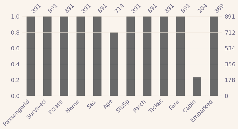
msno.bar(titanic)
fig = plt.gcf()
fig.set_size_inches(10, 4)
plt.show()
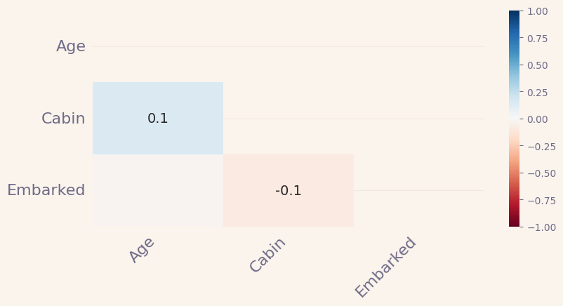
msno.heatmap(titanic)
fig = plt.gcf()
fig.set_size_inches(9, 4)
plt.show()
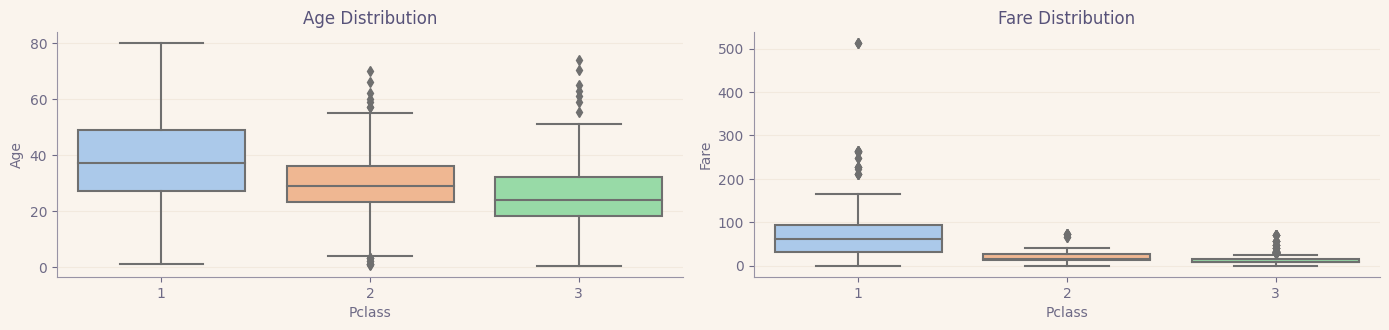
plt.figure(figsize=(14,len(num_cols)*3))
for idx,column in enumerate(num_cols):
    plt.subplot(len(num_cols)//2+1,2,idx+1)
    sns.boxplot(x="Pclass", y=column, data=titanic,palette="pastel")
    plt.title(f"{column} Distribution")
    plt.tight_layout()
missing_cols = missing_values_table(titanic, True)
|          |   n_miss |   ratio |
|:---------|---------:|--------:|
| Cabin    |      687 |   77.1  |
| Age      |      177 |   19.87 |
| Embarked |        2 |    0.22 |
missing_cols
['Age', 'Cabin', 'Embarked']
def missing_vs_target(dataframe, target, na_columns):

    temp_df = dataframe.copy()

    for col in na_columns:

        temp_df[col + '_NA_FLAG'] = np.where(temp_df[col].isnull(), 1, 0)

    na_flags = temp_df.loc[:, temp_df.columns.str.contains("_NA_")].columns

    for col in na_flags:

        result_df = pd.DataFrame({"TARGET_MEAN": temp_df.groupby(col)[target].mean(),
                                  "Count": temp_df.groupby(col)[target].count()})
        print(result_df.to_markdown(), end="\n\n\n")
missing_vs_target(titanic, "Survived", missing_cols)
|   Age_NA_FLAG |   TARGET_MEAN |   Count |
|--------------:|--------------:|--------:|
|             0 |      0.406162 |     714 |
|             1 |      0.293785 |     177 |


|   Cabin_NA_FLAG |   TARGET_MEAN |   Count |
|----------------:|--------------:|--------:|
|               0 |      0.666667 |     204 |
|               1 |      0.299854 |     687 |


|   Embarked_NA_FLAG |   TARGET_MEAN |   Count |
|-------------------:|--------------:|--------:|
|                  0 |      0.382452 |     889 |
|                  1 |      1        |       2 |
🗨️ Comment:
- 在这里,"1"代表有缺失值的人,"0"代表没有缺失值的人。
- 如果我们看一下Age_NA_FLAG的值,那些有缺失值的人的平均生存率为"0.293785",而那些有完整年龄值的人的生存率为"0.406162"。
- 让我们来看一下Cabin_NA_FLAG变量;这个变量有77.1%的缺失值率。有缺失值的观测的生存率为"0.299854",而没有缺失值的观测的生存率为"0.666667"。存在显著差异。
- 实际上,这背后有一个普遍的故事;"Cabin"变量中缺失值如此之高的一个原因可能是许多船员没有舱位号。他们没有被分配这样的值,因为他们不住在舱房里。大多数住在舱房里的人是乘客。可以推断出一些这些缺失值属于船员。
- 所有这些评论都是为了进行分析和解释的尝试。
编码
编码是一种数据预处理技术,用于将分类数据转换为数值格式。分类数据是以文本或符号为基础的数据,许多机器学习算法无法处理此类数据。以下是常用的编码方法:
-
标签编码:该方法为每个不同的类别分配一个唯一的数字。例如,类别"红色"、"蓝色"和"绿色"被编码为0、1和2。标签编码适用于有序分类数据,其中数据的顺序很重要。
-
独热编码:该方法为每个类别创建一列,并在每个观察值的每个列中分配值1或0。例如,对于类别"红色"、“蓝色"和"绿色”,将创建三个单独的列。一个观察值如果是"红色",则在"红色"列中的值为1,在其他列中的值为0。独热编码适用于名义分类数据,其中没有固有的顺序。
-
稀有编码:该方法将罕见或低频的分类值组合起来。它特别适用于具有大量不同类别的变量。稀有编码将罕见的类别归为一个"稀有"类别,同时保留其他类别。这有助于模型更好地学习罕见类别。
选择编码方法取决于数据的特性和特定的预处理要求。选择正确的编码方法和参数是数据预处理的关键部分,因为它可以显著影响模型的性能。
在使用编码方法时,有几个重要的参数需要考虑:
-
类别数量: 在对分类变量进行编码之前,了解有多少不同的类别是至关重要的。在使用独热编码时,大量的类别可能会导致许多列和增加的模型复杂性。罕见编码需要了解罕见类别的频率信息。
-
有序性: 如果数据是有序的(例如,“低”,“中”,“高”),可以使用标签编码。对于无序数据(例如,“红”,“蓝”,“绿”),独热编码可能是一个更好的选择。
-
区分能力: 分类变量的区分能力决定了一个类别对目标变量的影响程度。这在使用罕见编码时尤为重要,因为罕见类别可能对目标变量产生强烈影响。
-
罕见编码阈值: 在使用罕见编码时,需要选择一个被认为是“罕见”的阈值,并将其合并到“罕见”类别下。这个阈值可以根据数据的结构和问题领域的不同而变化。
-
独热编码虚拟变量陷阱: 在使用独热编码时,使用“drop_first”参数是非常重要的,可以合并表示相同类别的列,并避免虚拟变量陷阱。
-
标签编码与目标变量的关系: 在使用标签编码时,要考虑分类变量与目标变量之间的关系。如果没有或关系较弱,使用标签编码的效果可能会受限。
✨Label Encoding✨
titanic = titanic_.copy()
titanic["Sex"].head()
0      male
1    female
2    female
3    female
4      male
Name: Sex, dtype: object
🗨️ Comment:
- 对于机器学习,我们需要将“男性”和“女性”的观察结果转化为数学表达式(二进制)。
le = LabelEncoder()
le.fit_transform(titanic["Sex"])[0:5]
array([1, 0, 0, 0, 1])
# If we wonder about the equivalents of 0 and 1;

le.inverse_transform([0, 1])
array(['female', 'male'], dtype=object)
def label_encoder(dataframe, binary_col):

    labelencoder = LabelEncoder()
    dataframe[binary_col] = labelencoder.fit_transform(dataframe[binary_col])

    return dataframe
titanic = titanic_.copy()
binary_cols = [col for col in titanic.columns if titanic[col].dtype not in [int, float]
               and titanic[col].nunique() == 2]

binary_cols
['Sex']
titanic[binary_cols].head()
| Sex | |
|---|---|
| 0 | male |
| 1 | female |
| 2 | female |
| 3 | female |
| 4 | male |
for col in binary_cols:

    label_encoder(titanic, col)

titanic. head()
| PassengerId | Survived | Pclass | Name | Sex | Age | SibSp | Parch | Ticket | Fare | Cabin | Embarked | |
|---|---|---|---|---|---|---|---|---|---|---|---|---|
| 0 | 1 | 0 | 3 | Braund, Mr. Owen Harris | 1 | 22.0 | 1 | 0 | A/5 21171 | 7.2500 | NaN | S |
| 1 | 2 | 1 | 1 | Cumings, Mrs. John Bradley (Florence Briggs Th... | 0 | 38.0 | 1 | 0 | PC 17599 | 71.2833 | C85 | C |
| 2 | 3 | 1 | 3 | Heikkinen, Miss. Laina | 0 | 26.0 | 0 | 0 | STON/O2. 3101282 | 7.9250 | NaN | S |
| 3 | 4 | 1 | 1 | Futrelle, Mrs. Jacques Heath (Lily May Peel) | 0 | 35.0 | 1 | 0 | 113803 | 53.1000 | C123 | S |
| 4 | 5 | 0 | 3 | Allen, Mr. William Henry | 1 | 35.0 | 0 | 0 | 373450 | 8.0500 | NaN | S |
✨One Hot Encoding✨
titanic = titanic_.copy()
titanic["Embarked"].value_counts()
Embarked
S    644
C    168
Q     77
Name: count, dtype: int64
pd.get_dummies(titanic, columns=["Embarked"], drop_first=True).head()
| PassengerId | Survived | Pclass | Name | Sex | Age | SibSp | Parch | Ticket | Fare | Cabin | Embarked_Q | Embarked_S | |
|---|---|---|---|---|---|---|---|---|---|---|---|---|---|
| 0 | 1 | 0 | 3 | Braund, Mr. Owen Harris | male | 22.0 | 1 | 0 | A/5 21171 | 7.2500 | NaN | False | True |
| 1 | 2 | 1 | 1 | Cumings, Mrs. John Bradley (Florence Briggs Th... | female | 38.0 | 1 | 0 | PC 17599 | 71.2833 | C85 | False | False |
| 2 | 3 | 1 | 3 | Heikkinen, Miss. Laina | female | 26.0 | 0 | 0 | STON/O2. 3101282 | 7.9250 | NaN | False | True |
| 3 | 4 | 1 | 1 | Futrelle, Mrs. Jacques Heath (Lily May Peel) | female | 35.0 | 1 | 0 | 113803 | 53.1000 | C123 | False | True |
| 4 | 5 | 0 | 3 | Allen, Mr. William Henry | male | 35.0 | 0 | 0 | 373450 | 8.0500 | NaN | False | True |
🗨️ Comment:
- 为了避免虚拟变量陷阱,变量之间不应该可以从彼此生成,我们使用“drop_first = True”来删除第一个类别。
pd.get_dummies(titanic, columns=["Embarked"], dummy_na=True).head()
| PassengerId | Survived | Pclass | Name | Sex | Age | SibSp | Parch | Ticket | Fare | Cabin | Embarked_C | Embarked_Q | Embarked_S | Embarked_nan | |
|---|---|---|---|---|---|---|---|---|---|---|---|---|---|---|---|
| 0 | 1 | 0 | 3 | Braund, Mr. Owen Harris | male | 22.0 | 1 | 0 | A/5 21171 | 7.2500 | NaN | False | False | True | False |
| 1 | 2 | 1 | 1 | Cumings, Mrs. John Bradley (Florence Briggs Th... | female | 38.0 | 1 | 0 | PC 17599 | 71.2833 | C85 | True | False | False | False |
| 2 | 3 | 1 | 3 | Heikkinen, Miss. Laina | female | 26.0 | 0 | 0 | STON/O2. 3101282 | 7.9250 | NaN | False | False | True | False |
| 3 | 4 | 1 | 1 | Futrelle, Mrs. Jacques Heath (Lily May Peel) | female | 35.0 | 1 | 0 | 113803 | 53.1000 | C123 | False | False | True | False |
| 4 | 5 | 0 | 3 | Allen, Mr. William Henry | male | 35.0 | 0 | 0 | 373450 | 8.0500 | NaN | False | False | True | False |
🗨️ Comment:
- 如果我们希望将变量中的缺失值视为一个类别,我们可以使用“dummy_na = True”。
pd.get_dummies(titanic, columns=["Sex", "Embarked"], drop_first=True).head()
| PassengerId | Survived | Pclass | Name | Age | SibSp | Parch | Ticket | Fare | Cabin | Sex_male | Embarked_Q | Embarked_S | |
|---|---|---|---|---|---|---|---|---|---|---|---|---|---|
| 0 | 1 | 0 | 3 | Braund, Mr. Owen Harris | 22.0 | 1 | 0 | A/5 21171 | 7.2500 | NaN | True | False | True |
| 1 | 2 | 1 | 1 | Cumings, Mrs. John Bradley (Florence Briggs Th... | 38.0 | 1 | 0 | PC 17599 | 71.2833 | C85 | False | False | False |
| 2 | 3 | 1 | 3 | Heikkinen, Miss. Laina | 26.0 | 0 | 0 | STON/O2. 3101282 | 7.9250 | NaN | False | False | True |
| 3 | 4 | 1 | 1 | Futrelle, Mrs. Jacques Heath (Lily May Peel) | 35.0 | 1 | 0 | 113803 | 53.1000 | C123 | False | False | True |
| 4 | 5 | 0 | 3 | Allen, Mr. William Henry | 35.0 | 0 | 0 | 373450 | 8.0500 | NaN | True | False | True |
def one_hot_encoder(dataframe, categorical_cols, drop_first=True):

    dataframe = pd.get_dummies(dataframe, columns=categorical_cols, drop_first=drop_first)

    return dataframe
cat_cols, num_cols, cat_but_car = grab_col_names(titanic)
Observations: 891
Variables: 12
cat_cols: 6
num_cols: 3
cat_but_car: 3
num_but_cat: 4
cat_cols
['Sex', 'Embarked', 'Survived', 'Pclass', 'SibSp', 'Parch']
ohe_cols = [col for col in titanic.columns if 10 >= titanic[col].nunique() > 2] # one-hot-encoding cols
ohe_cols
['Pclass', 'SibSp', 'Parch', 'Embarked']
one_hot_encoder(titanic, ohe_cols).head() # to make a permanent change, it should be assigned to "titanic."
| PassengerId | Survived | Name | Sex | Age | Ticket | Fare | Cabin | Pclass_2 | Pclass_3 | ... | SibSp_5 | SibSp_8 | Parch_1 | Parch_2 | Parch_3 | Parch_4 | Parch_5 | Parch_6 | Embarked_Q | Embarked_S | |
|---|---|---|---|---|---|---|---|---|---|---|---|---|---|---|---|---|---|---|---|---|---|
| 0 | 1 | 0 | Braund, Mr. Owen Harris | male | 22.0 | A/5 21171 | 7.2500 | NaN | False | True | ... | False | False | False | False | False | False | False | False | False | True |
| 1 | 2 | 1 | Cumings, Mrs. John Bradley (Florence Briggs Th... | female | 38.0 | PC 17599 | 71.2833 | C85 | False | False | ... | False | False | False | False | False | False | False | False | False | False |
| 2 | 3 | 1 | Heikkinen, Miss. Laina | female | 26.0 | STON/O2. 3101282 | 7.9250 | NaN | False | True | ... | False | False | False | False | False | False | False | False | False | True |
| 3 | 4 | 1 | Futrelle, Mrs. Jacques Heath (Lily May Peel) | female | 35.0 | 113803 | 53.1000 | C123 | False | False | ... | False | False | False | False | False | False | False | False | False | True |
| 4 | 5 | 0 | Allen, Mr. William Henry | male | 35.0 | 373450 | 8.0500 | NaN | False | True | ... | False | False | False | False | False | False | False | False | False | True |
5 rows × 24 columns
titanic.head()
| PassengerId | Survived | Pclass | Name | Sex | Age | SibSp | Parch | Ticket | Fare | Cabin | Embarked | |
|---|---|---|---|---|---|---|---|---|---|---|---|---|
| 0 | 1 | 0 | 3 | Braund, Mr. Owen Harris | male | 22.0 | 1 | 0 | A/5 21171 | 7.2500 | NaN | S |
| 1 | 2 | 1 | 1 | Cumings, Mrs. John Bradley (Florence Briggs Th... | female | 38.0 | 1 | 0 | PC 17599 | 71.2833 | C85 | C |
| 2 | 3 | 1 | 3 | Heikkinen, Miss. Laina | female | 26.0 | 0 | 0 | STON/O2. 3101282 | 7.9250 | NaN | S |
| 3 | 4 | 1 | 1 | Futrelle, Mrs. Jacques Heath (Lily May Peel) | female | 35.0 | 1 | 0 | 113803 | 53.1000 | C123 | S |
| 4 | 5 | 0 | 3 | Allen, Mr. William Henry | male | 35.0 | 0 | 0 | 373450 | 8.0500 | NaN | S |
✨Rare Encoding✨
基于出现频率分析分类变量;
home_credit["NAME_EDUCATION_TYPE"].value_counts()
NAME_EDUCATION_TYPE
Secondary / secondary special    218391
Higher education                  74863
Incomplete higher                 10277
Lower secondary                    3816
Academic degree                     164
Name: count, dtype: int64
cat_cols, num_cols, cat_but_car = grab_col_names(home_credit)
Observations: 307511
Variables: 122
cat_cols: 54
num_cols: 67
cat_but_car: 1
num_but_cat: 39
def cat_summary(dataframe, col_name, plot=False):

    summary_df = pd.DataFrame({col_name: dataframe[col_name].value_counts(),
                               "Ratio": 100 * dataframe[col_name].value_counts() / len(dataframe)})

    print(summary_df.to_markdown(), end="\n\n")

    if plot:

        sns.countplot(x=dataframe[col_name], data=dataframe)
        plt.show()
for col in cat_cols:

    cat_summary(home_credit, col)
| NAME_CONTRACT_TYPE | NAME_CONTRACT_TYPE | Ratio |
|:---------------------|---------------------:|---------:|
| Cash loans | 278232 | 90.4787 |
| Revolving loans | 29279 | 9.52129 |
| CODE_GENDER | CODE_GENDER | Ratio |
|:--------------|--------------:|------------:|
| F | 202448 | 65.8344 |
| M | 105059 | 34.1643 |
| XNA | 4 | 0.00130077 |
| FLAG_OWN_CAR | FLAG_OWN_CAR | Ratio |
|:---------------|---------------:|--------:|
| N | 202924 | 65.9892 |
| Y | 104587 | 34.0108 |
| FLAG_OWN_REALTY | FLAG_OWN_REALTY | Ratio |
|:------------------|------------------:|--------:|
| Y | 213312 | 69.3673 |
| N | 94199 | 30.6327 |
| NAME_TYPE_SUITE | NAME_TYPE_SUITE | Ratio |
|:------------------|------------------:|-----------:|
| Unaccompanied | 248526 | 80.8186 |
| Family | 40149 | 13.0561 |
| Spouse, partner | 11370 | 3.69743 |
| Children | 3267 | 1.0624 |
| Other_B | 1770 | 0.575589 |
| Other_A | 866 | 0.281616 |
| Group of people | 271 | 0.0881269 |
| NAME_INCOME_TYPE | NAME_INCOME_TYPE | Ratio |
|:---------------------|-------------------:|------------:|
| Working | 158774 | 51.632 |
| Commercial associate | 71617 | 23.2892 |
| Pensioner | 55362 | 18.0033 |
| State servant | 21703 | 7.05763 |
| Unemployed | 22 | 0.00715422 |
| Student | 18 | 0.00585345 |
| Businessman | 10 | 0.00325192 |
| Maternity leave | 5 | 0.00162596 |
| NAME_EDUCATION_TYPE | NAME_EDUCATION_TYPE | Ratio |
|:------------------------------|----------------------:|-----------:|
| Secondary / secondary special | 218391 | 71.0189 |
| Higher education | 74863 | 24.3448 |
| Incomplete higher | 10277 | 3.34199 |
| Lower secondary | 3816 | 1.24093 |
| Academic degree | 164 | 0.0533314 |
| NAME_FAMILY_STATUS | NAME_FAMILY_STATUS | Ratio |
|:---------------------|---------------------:|-------------:|
| Married | 196432 | 63.878 |
| Single / not married | 45444 | 14.778 |
| Civil marriage | 29775 | 9.68258 |
| Separated | 19770 | 6.42904 |
| Widow | 16088 | 5.23168 |
| Unknown | 2 | 0.000650383 |
| NAME_HOUSING_TYPE | NAME_HOUSING_TYPE | Ratio |
|:--------------------|--------------------:|----------:|
| House / apartment | 272868 | 88.7344 |
| With parents | 14840 | 4.82584 |
| Municipal apartment | 11183 | 3.63662 |
| Rented apartment | 4881 | 1.58726 |
| Office apartment | 2617 | 0.851026 |
| Co-op apartment | 1122 | 0.364865 |
| OCCUPATION_TYPE | OCCUPATION_TYPE | Ratio |
|:----------------------|------------------:|----------:|
| Laborers | 55186 | 17.946 |
| Sales staff | 32102 | 10.4393 |
| Core staff | 27570 | 8.96553 |
| Managers | 21371 | 6.94967 |
| Drivers | 18603 | 6.04954 |
| High skill tech staff | 11380 | 3.70068 |
| Accountants | 9813 | 3.19111 |
| Medicine staff | 8537 | 2.77616 |
| Security staff | 6721 | 2.18561 |
| Cooking staff | 5946 | 1.93359 |
| Cleaning staff | 4653 | 1.51312 |
| Private service staff | 2652 | 0.862408 |
| Low-skill Laborers | 2093 | 0.680626 |
| Waiters/barmen staff | 1348 | 0.438358 |
| Secretaries | 1305 | 0.424375 |
| Realty agents | 751 | 0.244219 |
| HR staff | 563 | 0.183083 |
| IT staff | 526 | 0.171051 |
| WEEKDAY_APPR_PROCESS_START | WEEKDAY_APPR_PROCESS_START | Ratio |
|:-----------------------------|-----------------------------:|---------:|
| TUESDAY | 53901 | 17.5282 |
| WEDNESDAY | 51934 | 16.8885 |
| MONDAY | 50714 | 16.4918 |
| THURSDAY | 50591 | 16.4518 |
| FRIDAY | 50338 | 16.3695 |
| SATURDAY | 33852 | 11.0084 |
| SUNDAY | 16181 | 5.26193 |
| FONDKAPREMONT_MODE | FONDKAPREMONT_MODE | Ratio |
|:----------------------|---------------------:|---------:|
| reg oper account | 73830 | 24.0089 |
| reg oper spec account | 12080 | 3.92831 |
| not specified | 5687 | 1.84936 |
| org spec account | 5619 | 1.82725 |
| HOUSETYPE_MODE | HOUSETYPE_MODE | Ratio |
|:-----------------|-----------------:|----------:|
| block of flats | 150503 | 48.9423 |
| specific housing | 1499 | 0.487462 |
| terraced house | 1212 | 0.394132 |
| WALLSMATERIAL_MODE | WALLSMATERIAL_MODE | Ratio |
|:---------------------|---------------------:|----------:|
| Panel | 66040 | 21.4757 |
| Stone, brick | 64815 | 21.0773 |
| Block | 9253 | 3.009 |
| Wooden | 5362 | 1.74368 |
| Mixed | 2296 | 0.74664 |
| Monolithic | 1779 | 0.578516 |
| Others | 1625 | 0.528436 |
| EMERGENCYSTATE_MODE | EMERGENCYSTATE_MODE | Ratio |
|:----------------------|----------------------:|----------:|
| No | 159428 | 51.8446 |
| Yes | 2328 | 0.757046 |
| TARGET | TARGET | Ratio |
|---------:|---------:|---------:|
| 0 | 282686 | 91.9271 |
| 1 | 24825 | 8.07288 |
| FLAG_MOBIL | FLAG_MOBIL | Ratio |
|-------------:|-------------:|-------------:|
| 1 | 307510 | 99.9997 |
| 0 | 1 | 0.000325192 |
| FLAG_EMP_PHONE | FLAG_EMP_PHONE | Ratio |
|-----------------:|-----------------:|--------:|
| 1 | 252125 | 81.9889 |
| 0 | 55386 | 18.0111 |
| FLAG_WORK_PHONE | FLAG_WORK_PHONE | Ratio |
|------------------:|------------------:|--------:|
| 0 | 246203 | 80.0632 |
| 1 | 61308 | 19.9368 |
| FLAG_CONT_MOBILE | FLAG_CONT_MOBILE | Ratio |
|-------------------:|-------------------:|---------:|
| 1 | 306937 | 99.8133 |
| 0 | 574 | 0.18666 |
| FLAG_PHONE | FLAG_PHONE | Ratio |
|-------------:|-------------:|--------:|
| 0 | 221080 | 71.8934 |
| 1 | 86431 | 28.1066 |
| FLAG_EMAIL | FLAG_EMAIL | Ratio |
|-------------:|-------------:|---------:|
| 0 | 290069 | 94.328 |
| 1 | 17442 | 5.67199 |
| REGION_RATING_CLIENT | REGION_RATING_CLIENT | Ratio |
|-----------------------:|-----------------------:|--------:|
| 2 | 226984 | 73.8133 |
| 3 | 48330 | 15.7165 |
| 1 | 32197 | 10.4702 |
| REGION_RATING_CLIENT_W_CITY | REGION_RATING_CLIENT_W_CITY | Ratio |
|------------------------------:|------------------------------:|--------:|
| 2 | 229484 | 74.6263 |
| 3 | 43860 | 14.2629 |
| 1 | 34167 | 11.1108 |
| REG_REGION_NOT_LIVE_REGION | REG_REGION_NOT_LIVE_REGION | Ratio |
|-----------------------------:|-----------------------------:|---------:|
| 0 | 302854 | 98.4856 |
| 1 | 4657 | 1.51442 |
| REG_REGION_NOT_WORK_REGION | REG_REGION_NOT_WORK_REGION | Ratio |
|-----------------------------:|-----------------------------:|---------:|
| 0 | 291899 | 94.9231 |
| 1 | 15612 | 5.07689 |
| LIVE_REGION_NOT_WORK_REGION | LIVE_REGION_NOT_WORK_REGION | Ratio |
|------------------------------:|------------------------------:|---------:|
| 0 | 295008 | 95.9341 |
| 1 | 12503 | 4.06587 |
| REG_CITY_NOT_LIVE_CITY | REG_CITY_NOT_LIVE_CITY | Ratio |
|-------------------------:|-------------------------:|---------:|
| 0 | 283472 | 92.1827 |
| 1 | 24039 | 7.81728 |
| REG_CITY_NOT_WORK_CITY | REG_CITY_NOT_WORK_CITY | Ratio |
|-------------------------:|-------------------------:|--------:|
| 0 | 236644 | 76.9546 |
| 1 | 70867 | 23.0454 |
| LIVE_CITY_NOT_WORK_CITY | LIVE_CITY_NOT_WORK_CITY | Ratio |
|--------------------------:|--------------------------:|--------:|
| 0 | 252296 | 82.0445 |
| 1 | 55215 | 17.9555 |
| DEF_60_CNT_SOCIAL_CIRCLE | DEF_60_CNT_SOCIAL_CIRCLE | Ratio |
|---------------------------:|---------------------------:|-------------:|
| 0 | 280721 | 91.2881 |
| 1 | 21841 | 7.10251 |
| 2 | 3170 | 1.03086 |
| 3 | 598 | 0.194465 |
| 4 | 135 | 0.0439009 |
| 5 | 20 | 0.00650383 |
| 6 | 3 | 0.000975575 |
| 7 | 1 | 0.000325192 |
| 24 | 1 | 0.000325192 |
| FLAG_DOCUMENT_2 | FLAG_DOCUMENT_2 | Ratio |
|------------------:|------------------:|------------:|
| 0 | 307498 | 99.9958 |
| 1 | 13 | 0.00422749 |
| FLAG_DOCUMENT_3 | FLAG_DOCUMENT_3 | Ratio |
|------------------:|------------------:|--------:|
| 1 | 218340 | 71.0023 |
| 0 | 89171 | 28.9977 |
| FLAG_DOCUMENT_4 | FLAG_DOCUMENT_4 | Ratio |
|------------------:|------------------:|------------:|
| 0 | 307486 | 99.9919 |
| 1 | 25 | 0.00812979 |
| FLAG_DOCUMENT_5 | FLAG_DOCUMENT_5 | Ratio |
|------------------:|------------------:|---------:|
| 0 | 302863 | 98.4885 |
| 1 | 4648 | 1.51149 |
| FLAG_DOCUMENT_6 | FLAG_DOCUMENT_6 | Ratio |
|------------------:|------------------:|---------:|
| 0 | 280433 | 91.1945 |
| 1 | 27078 | 8.80554 |
| FLAG_DOCUMENT_7 | FLAG_DOCUMENT_7 | Ratio |
|------------------:|------------------:|-----------:|
| 0 | 307452 | 99.9808 |
| 1 | 59 | 0.0191863 |
| FLAG_DOCUMENT_8 | FLAG_DOCUMENT_8 | Ratio |
|------------------:|------------------:|--------:|
| 0 | 282487 | 91.8624 |
| 1 | 25024 | 8.1376 |
| FLAG_DOCUMENT_9 | FLAG_DOCUMENT_9 | Ratio |
|------------------:|------------------:|---------:|
| 0 | 306313 | 99.6104 |
| 1 | 1198 | 0.38958 |
| FLAG_DOCUMENT_10 | FLAG_DOCUMENT_10 | Ratio |
|-------------------:|-------------------:|------------:|
| 0 | 307504 | 99.9977 |
| 1 | 7 | 0.00227634 |
| FLAG_DOCUMENT_11 | FLAG_DOCUMENT_11 | Ratio |
|-------------------:|-------------------:|----------:|
| 0 | 306308 | 99.6088 |
| 1 | 1203 | 0.391206 |
| FLAG_DOCUMENT_12 | FLAG_DOCUMENT_12 | Ratio |
|-------------------:|-------------------:|-------------:|
| 0 | 307509 | 99.9993 |
| 1 | 2 | 0.000650383 |
| FLAG_DOCUMENT_13 | FLAG_DOCUMENT_13 | Ratio |
|-------------------:|-------------------:|----------:|
| 0 | 306427 | 99.6475 |
| 1 | 1084 | 0.352508 |
| FLAG_DOCUMENT_14 | FLAG_DOCUMENT_14 | Ratio |
|-------------------:|-------------------:|----------:|
| 0 | 306608 | 99.7064 |
| 1 | 903 | 0.293648 |
| FLAG_DOCUMENT_15 | FLAG_DOCUMENT_15 | Ratio |
|-------------------:|-------------------:|----------:|
| 0 | 307139 | 99.879 |
| 1 | 372 | 0.120971 |
| FLAG_DOCUMENT_16 | FLAG_DOCUMENT_16 | Ratio |
|-------------------:|-------------------:|---------:|
| 0 | 304458 | 99.0072 |
| 1 | 3053 | 0.99281 |
| FLAG_DOCUMENT_17 | FLAG_DOCUMENT_17 | Ratio |
|-------------------:|-------------------:|-----------:|
| 0 | 307429 | 99.9733 |
| 1 | 82 | 0.0266657 |
| FLAG_DOCUMENT_18 | FLAG_DOCUMENT_18 | Ratio |
|-------------------:|-------------------:|----------:|
| 0 | 305011 | 99.187 |
| 1 | 2500 | 0.812979 |
| FLAG_DOCUMENT_19 | FLAG_DOCUMENT_19 | Ratio |
|-------------------:|-------------------:|-----------:|
| 0 | 307328 | 99.9405 |
| 1 | 183 | 0.0595101 |
| FLAG_DOCUMENT_20 | FLAG_DOCUMENT_20 | Ratio |
|-------------------:|-------------------:|-----------:|
| 0 | 307355 | 99.9493 |
| 1 | 156 | 0.0507299 |
| FLAG_DOCUMENT_21 | FLAG_DOCUMENT_21 | Ratio |
|-------------------:|-------------------:|-----------:|
| 0 | 307408 | 99.9665 |
| 1 | 103 | 0.0334947 |
| AMT_REQ_CREDIT_BUREAU_HOUR | AMT_REQ_CREDIT_BUREAU_HOUR | Ratio |
|-----------------------------:|-----------------------------:|-------------:|
| 0 | 264366 | 85.9696 |
| 1 | 1560 | 0.507299 |
| 2 | 56 | 0.0182107 |
| 3 | 9 | 0.00292672 |
| 4 | 1 | 0.000325192 |
| AMT_REQ_CREDIT_BUREAU_DAY | AMT_REQ_CREDIT_BUREAU_DAY | Ratio |
|----------------------------:|----------------------------:|-------------:|
| 0 | 264503 | 86.0142 |
| 1 | 1292 | 0.420148 |
| 2 | 106 | 0.0344703 |
| 3 | 45 | 0.0146336 |
| 4 | 26 | 0.00845498 |
| 5 | 9 | 0.00292672 |
| 6 | 8 | 0.00260153 |
| 9 | 2 | 0.000650383 |
| 8 | 1 | 0.000325192 |
| AMT_REQ_CREDIT_BUREAU_WEEK | AMT_REQ_CREDIT_BUREAU_WEEK | Ratio |
|-----------------------------:|-----------------------------:|-------------:|
| 0 | 257456 | 83.7225 |
| 1 | 8208 | 2.66917 |
| 2 | 199 | 0.0647131 |
| 3 | 58 | 0.0188611 |
| 4 | 34 | 0.0110565 |
| 6 | 20 | 0.00650383 |
| 5 | 10 | 0.00325192 |
| 8 | 5 | 0.00162596 |
| 7 | 2 | 0.000650383 |
🗨️ Comment:
- 如图所示,有一些观察结果在变量中出现的概率非常低。我们可以将这些低频观察结果分组,并进行编码,而不是对所有这些值应用独热编码。
Analyzing the relationship between rare categories and the dependent variable;
home_credit["NAME_INCOME_TYPE"].value_counts()
NAME_INCOME_TYPE
Working                 158774
Commercial associate     71617
Pensioner                55362
State servant            21703
Unemployed                  22
Student                     18
Businessman                 10
Maternity leave              5
Name: count, dtype: int64
🗨️ Comment:
我们可以考虑一些评论:
- 类别“失业、学生、商人和产假”可以被归为一个单一类别。
- 当然,在这一点上,个人意见会起到作用。在机器学习之前进行的这种合并可能被模型视为噪音。
- 相反,它也可能导致成功的建模结果。
- 在罕见编码过程中,谨慎行事并仔细监控个人决策非常重要。
home_credit.groupby("NAME_INCOME_TYPE")["TARGET"].mean()
NAME_INCOME_TYPE
Businessman             0.000000
Commercial associate    0.074843
Maternity leave         0.400000
Pensioner               0.053864
State servant           0.057550
Student                 0.000000
Unemployed              0.363636
Working                 0.095885
Name: TARGET, dtype: float64
def rare_analyser(dataframe, target, cat_cols):

    for col in cat_cols:

        print(f"{col} : {len(dataframe[col].value_counts())}\n")

        summary_df = pd.DataFrame({
            "COUNT": dataframe[col].value_counts(),
            "RATIO": dataframe[col].value_counts() / len(dataframe),
            "TARGET_MEAN": dataframe.groupby(col)[target].mean()
        })

        print(summary_df.to_markdown(), end="\n\n\n")
# rare_analyser(home_credit, "TARGET", cat_cols)
Rare Encoding Function;
def rare_encoder(dataframe, rare_perc):

    temp_df = dataframe.copy()

    rare_columns = [col for col in temp_df.columns if temp_df[col].dtypes == 'O'
                    and (temp_df[col].value_counts() / len(temp_df) < rare_perc).any(axis=None)]

    for var in rare_columns:

        tmp = temp_df[var].value_counts() / len(temp_df)
        rare_labels = tmp[tmp < rare_perc].index
        temp_df[var] = np.where(temp_df[var].isin(rare_labels), 'Rare', temp_df[var])

    return temp_df
new_df = rare_encoder(home_credit, 0.01)
rare_analyser(new_df, "TARGET", cat_cols)
NAME_CONTRACT_TYPE : 2
| NAME_CONTRACT_TYPE | COUNT | RATIO | TARGET_MEAN |
|:---------------------|--------:|----------:|--------------:|
| Cash loans | 278232 | 0.904787 | 0.0834591 |
| Revolving loans | 29279 | 0.0952129 | 0.0547833 |
CODE_GENDER : 3
| CODE_GENDER | COUNT | RATIO | TARGET_MEAN |
|:--------------|--------:|------------:|--------------:|
| F | 202448 | 0.658344 | 0.0699933 |
| M | 105059 | 0.341643 | 0.101419 |
| Rare | 4 | 1.30077e-05 | 0 |
FLAG_OWN_CAR : 2
| FLAG_OWN_CAR | COUNT | RATIO | TARGET_MEAN |
|:---------------|--------:|---------:|--------------:|
| N | 202924 | 0.659892 | 0.0850023 |
| Y | 104587 | 0.340108 | 0.0724373 |
FLAG_OWN_REALTY : 2
| FLAG_OWN_REALTY | COUNT | RATIO | TARGET_MEAN |
|:------------------|--------:|---------:|--------------:|
| N | 94199 | 0.306327 | 0.0832493 |
| Y | 213312 | 0.693673 | 0.0796158 |
NAME_TYPE_SUITE : 5
| NAME_TYPE_SUITE | COUNT | RATIO | TARGET_MEAN |
|:------------------|--------:|-----------:|--------------:|
| Children | 3267 | 0.010624 | 0.073768 |
| Family | 40149 | 0.130561 | 0.0749458 |
| Rare | 2907 | 0.00945332 | 0.0939112 |
| Spouse, partner | 11370 | 0.0369743 | 0.0787159 |
| Unaccompanied | 248526 | 0.808186 | 0.0818305 |
NAME_INCOME_TYPE : 5
| NAME_INCOME_TYPE | COUNT | RATIO | TARGET_MEAN |
|:---------------------|--------:|------------:|--------------:|
| Commercial associate | 71617 | 0.232892 | 0.0748426 |
| Pensioner | 55362 | 0.180033 | 0.0538637 |
| Rare | 55 | 0.000178855 | 0.181818 |
| State servant | 21703 | 0.0705763 | 0.0575496 |
| Working | 158774 | 0.51632 | 0.0958847 |
NAME_EDUCATION_TYPE : 5
| NAME_EDUCATION_TYPE | COUNT | RATIO | TARGET_MEAN |
|:------------------------------|--------:|------------:|--------------:|
| Higher education | 74863 | 0.243448 | 0.0535512 |
| Incomplete higher | 10277 | 0.0334199 | 0.0848497 |
| Lower secondary | 3816 | 0.0124093 | 0.109277 |
| Rare | 164 | 0.000533314 | 0.0182927 |
| Secondary / secondary special | 218391 | 0.710189 | 0.0893993 |
NAME_FAMILY_STATUS : 6
| NAME_FAMILY_STATUS | COUNT | RATIO | TARGET_MEAN |
|:---------------------|--------:|------------:|--------------:|
| Civil marriage | 29775 | 0.0968258 | 0.0994458 |
| Married | 196432 | 0.63878 | 0.0755987 |
| Rare | 2 | 6.50383e-06 | 0 |
| Separated | 19770 | 0.0642904 | 0.0819423 |
| Single / not married | 45444 | 0.14778 | 0.0980768 |
| Widow | 16088 | 0.0523168 | 0.0582422 |
NAME_HOUSING_TYPE : 5
| NAME_HOUSING_TYPE | COUNT | RATIO | TARGET_MEAN |
|:--------------------|--------:|----------:|--------------:|
| House / apartment | 272868 | 0.887344 | 0.0779571 |
| Municipal apartment | 11183 | 0.0363662 | 0.0853975 |
| Rare | 3739 | 0.0121589 | 0.0698048 |
| Rented apartment | 4881 | 0.0158726 | 0.123131 |
| With parents | 14840 | 0.0482584 | 0.116981 |
OCCUPATION_TYPE : 12
| OCCUPATION_TYPE | COUNT | RATIO | TARGET_MEAN |
|:----------------------|--------:|----------:|--------------:|
| Accountants | 9813 | 0.0319111 | 0.0483033 |
| Cleaning staff | 4653 | 0.0151312 | 0.0960671 |
| Cooking staff | 5946 | 0.0193359 | 0.10444 |
| Core staff | 27570 | 0.0896553 | 0.0630395 |
| Drivers | 18603 | 0.0604954 | 0.113261 |
| High skill tech staff | 11380 | 0.0370068 | 0.0615993 |
| Laborers | 55186 | 0.17946 | 0.105788 |
| Managers | 21371 | 0.0694967 | 0.0621403 |
| Medicine staff | 8537 | 0.0277616 | 0.0670025 |
| Rare | 9238 | 0.0300412 | 0.0981814 |
| Sales staff | 32102 | 0.104393 | 0.096318 |
| Security staff | 6721 | 0.0218561 | 0.107424 |
WEEKDAY_APPR_PROCESS_START : 7
| WEEKDAY_APPR_PROCESS_START | COUNT | RATIO | TARGET_MEAN |
|:-----------------------------|--------:|----------:|--------------:|
| FRIDAY | 50338 | 0.163695 | 0.0814693 |
| MONDAY | 50714 | 0.164918 | 0.0775723 |
| SATURDAY | 33852 | 0.110084 | 0.0788727 |
| SUNDAY | 16181 | 0.0526193 | 0.0792905 |
| THURSDAY | 50591 | 0.164518 | 0.0810025 |
| TUESDAY | 53901 | 0.175282 | 0.0835049 |
| WEDNESDAY | 51934 | 0.168885 | 0.0816036 |
FONDKAPREMONT_MODE : 4
| FONDKAPREMONT_MODE | COUNT | RATIO | TARGET_MEAN |
|:----------------------|--------:|----------:|--------------:|
| not specified | 5687 | 0.0184936 | 0.0754352 |
| org spec account | 5619 | 0.0182725 | 0.0581954 |
| reg oper account | 73830 | 0.240089 | 0.0697819 |
| reg oper spec account | 12080 | 0.0392831 | 0.0655629 |
HOUSETYPE_MODE : 2
| HOUSETYPE_MODE | COUNT | RATIO | TARGET_MEAN |
|:-----------------|--------:|-----------:|--------------:|
| Rare | 2711 | 0.00881594 | 0.0940612 |
| block of flats | 150503 | 0.489423 | 0.0694338 |
WALLSMATERIAL_MODE : 5
| WALLSMATERIAL_MODE | COUNT | RATIO | TARGET_MEAN |
|:---------------------|--------:|----------:|--------------:|
| Block | 9253 | 0.03009 | 0.0702475 |
| Panel | 66040 | 0.214757 | 0.0634767 |
| Rare | 5700 | 0.0185359 | 0.0687719 |
| Stone, brick | 64815 | 0.210773 | 0.0740569 |
| Wooden | 5362 | 0.0174368 | 0.0969787 |
EMERGENCYSTATE_MODE : 2
| EMERGENCYSTATE_MODE | COUNT | RATIO | TARGET_MEAN |
|:----------------------|--------:|-----------:|--------------:|
| No | 159428 | 0.518446 | 0.069649 |
| Rare | 2328 | 0.00757046 | 0.0957904 |
TARGET : 2
| TARGET | COUNT | RATIO | TARGET_MEAN |
|---------:|--------:|----------:|--------------:|
| 0 | 282686 | 0.919271 | 0 |
| 1 | 24825 | 0.0807288 | 1 |
FLAG_MOBIL : 2
| FLAG_MOBIL | COUNT | RATIO | TARGET_MEAN |
|-------------:|--------:|------------:|--------------:|
| 0 | 1 | 3.25192e-06 | 0 |
| 1 | 307510 | 0.999997 | 0.0807291 |
FLAG_EMP_PHONE : 2
| FLAG_EMP_PHONE | COUNT | RATIO | TARGET_MEAN |
|-----------------:|--------:|---------:|--------------:|
| 0 | 55386 | 0.180111 | 0.0540028 |
| 1 | 252125 | 0.819889 | 0.0865999 |
FLAG_WORK_PHONE : 2
| FLAG_WORK_PHONE | COUNT | RATIO | TARGET_MEAN |
|------------------:|--------:|---------:|--------------:|
| 0 | 246203 | 0.800632 | 0.0768512 |
| 1 | 61308 | 0.199368 | 0.0963006 |
FLAG_CONT_MOBILE : 2
| FLAG_CONT_MOBILE | COUNT | RATIO | TARGET_MEAN |
|-------------------:|--------:|----------:|--------------:|
| 0 | 574 | 0.0018666 | 0.0783972 |
| 1 | 306937 | 0.998133 | 0.0807332 |
FLAG_PHONE : 2
| FLAG_PHONE | COUNT | RATIO | TARGET_MEAN |
|-------------:|--------:|---------:|--------------:|
| 0 | 221080 | 0.718934 | 0.0847838 |
| 1 | 86431 | 0.281066 | 0.0703567 |
FLAG_EMAIL : 2
| FLAG_EMAIL | COUNT | RATIO | TARGET_MEAN |
|-------------:|--------:|----------:|--------------:|
| 0 | 290069 | 0.94328 | 0.0808463 |
| 1 | 17442 | 0.0567199 | 0.0787754 |
REGION_RATING_CLIENT : 3
| REGION_RATING_CLIENT | COUNT | RATIO | TARGET_MEAN |
|-----------------------:|--------:|---------:|--------------:|
| 1 | 32197 | 0.104702 | 0.0482032 |
| 2 | 226984 | 0.738133 | 0.078891 |
| 3 | 48330 | 0.157165 | 0.111028 |
REGION_RATING_CLIENT_W_CITY : 3
| REGION_RATING_CLIENT_W_CITY | COUNT | RATIO | TARGET_MEAN |
|------------------------------:|--------:|---------:|--------------:|
| 1 | 34167 | 0.111108 | 0.0484093 |
| 2 | 229484 | 0.746263 | 0.0791776 |
| 3 | 43860 | 0.142629 | 0.114022 |
REG_REGION_NOT_LIVE_REGION : 2
| REG_REGION_NOT_LIVE_REGION | COUNT | RATIO | TARGET_MEAN |
|-----------------------------:|--------:|----------:|--------------:|
| 0 | 302854 | 0.984856 | 0.0805405 |
| 1 | 4657 | 0.0151442 | 0.0929783 |
REG_REGION_NOT_WORK_REGION : 2
| REG_REGION_NOT_WORK_REGION | COUNT | RATIO | TARGET_MEAN |
|-----------------------------:|--------:|----------:|--------------:|
| 0 | 291899 | 0.949231 | 0.0802915 |
| 1 | 15612 | 0.0507689 | 0.088906 |
LIVE_REGION_NOT_WORK_REGION : 2
| LIVE_REGION_NOT_WORK_REGION | COUNT | RATIO | TARGET_MEAN |
|------------------------------:|--------:|----------:|--------------:|
| 0 | 295008 | 0.959341 | 0.0805707 |
| 1 | 12503 | 0.0406587 | 0.0844597 |
REG_CITY_NOT_LIVE_CITY : 2
| REG_CITY_NOT_LIVE_CITY | COUNT | RATIO | TARGET_MEAN |
|-------------------------:|--------:|----------:|--------------:|
| 0 | 283472 | 0.921827 | 0.0772069 |
| 1 | 24039 | 0.0781728 | 0.12226 |
REG_CITY_NOT_WORK_CITY : 2
| REG_CITY_NOT_WORK_CITY | COUNT | RATIO | TARGET_MEAN |
|-------------------------:|--------:|---------:|--------------:|
| 0 | 236644 | 0.769546 | 0.0731267 |
| 1 | 70867 | 0.230454 | 0.106114 |
LIVE_CITY_NOT_WORK_CITY : 2
| LIVE_CITY_NOT_WORK_CITY | COUNT | RATIO | TARGET_MEAN |
|--------------------------:|--------:|---------:|--------------:|
| 0 | 252296 | 0.820445 | 0.0765846 |
| 1 | 55215 | 0.179555 | 0.0996649 |
DEF_60_CNT_SOCIAL_CIRCLE : 9
| DEF_60_CNT_SOCIAL_CIRCLE | COUNT | RATIO | TARGET_MEAN |
|---------------------------:|--------:|------------:|--------------:|
| 0 | 280721 | 0.912881 | 0.0783483 |
| 1 | 21841 | 0.0710251 | 0.105169 |
| 2 | 3170 | 0.0103086 | 0.121451 |
| 3 | 598 | 0.00194465 | 0.158863 |
| 4 | 135 | 0.000439009 | 0.111111 |
| 5 | 20 | 6.50383e-05 | 0.15 |
| 6 | 3 | 9.75575e-06 | 0 |
| 7 | 1 | 3.25192e-06 | 0 |
| 24 | 1 | 3.25192e-06 | 0 |
FLAG_DOCUMENT_2 : 2
| FLAG_DOCUMENT_2 | COUNT | RATIO | TARGET_MEAN |
|------------------:|--------:|------------:|--------------:|
| 0 | 307498 | 0.999958 | 0.0807192 |
| 1 | 13 | 4.22749e-05 | 0.307692 |
FLAG_DOCUMENT_3 : 2
| FLAG_DOCUMENT_3 | COUNT | RATIO | TARGET_MEAN |
|------------------:|--------:|---------:|--------------:|
| 0 | 89171 | 0.289977 | 0.061825 |
| 1 | 218340 | 0.710023 | 0.0884492 |
FLAG_DOCUMENT_4 : 2
| FLAG_DOCUMENT_4 | COUNT | RATIO | TARGET_MEAN |
|------------------:|--------:|------------:|--------------:|
| 0 | 307486 | 0.999919 | 0.0807354 |
| 1 | 25 | 8.12979e-05 | 0 |
FLAG_DOCUMENT_5 : 2
| FLAG_DOCUMENT_5 | COUNT | RATIO | TARGET_MEAN |
|------------------:|--------:|----------:|--------------:|
| 0 | 302863 | 0.984885 | 0.0807395 |
| 1 | 4648 | 0.0151149 | 0.0800344 |
FLAG_DOCUMENT_6 : 2
| FLAG_DOCUMENT_6 | COUNT | RATIO | TARGET_MEAN |
|------------------:|--------:|----------:|--------------:|
| 0 | 280433 | 0.911945 | 0.08315 |
| 1 | 27078 | 0.0880554 | 0.055654 |
FLAG_DOCUMENT_7 : 2
| FLAG_DOCUMENT_7 | COUNT | RATIO | TARGET_MEAN |
|------------------:|--------:|------------:|--------------:|
| 0 | 307452 | 0.999808 | 0.0807346 |
| 1 | 59 | 0.000191863 | 0.0508475 |
FLAG_DOCUMENT_8 : 2
| FLAG_DOCUMENT_8 | COUNT | RATIO | TARGET_MEAN |
|------------------:|--------:|---------:|--------------:|
| 0 | 282487 | 0.918624 | 0.0813807 |
| 1 | 25024 | 0.081376 | 0.0733696 |
FLAG_DOCUMENT_9 : 2
| FLAG_DOCUMENT_9 | COUNT | RATIO | TARGET_MEAN |
|------------------:|--------:|----------:|--------------:|
| 0 | 306313 | 0.996104 | 0.080803 |
| 1 | 1198 | 0.0038958 | 0.0617696 |
FLAG_DOCUMENT_10 : 2
| FLAG_DOCUMENT_10 | COUNT | RATIO | TARGET_MEAN |
|-------------------:|--------:|------------:|--------------:|
| 0 | 307504 | 0.999977 | 0.0807307 |
| 1 | 7 | 2.27634e-05 | 0 |
FLAG_DOCUMENT_11 : 2
| FLAG_DOCUMENT_11 | COUNT | RATIO | TARGET_MEAN |
|-------------------:|--------:|-----------:|--------------:|
| 0 | 306308 | 0.996088 | 0.080801 |
| 1 | 1203 | 0.00391206 | 0.0623441 |
FLAG_DOCUMENT_12 : 2
| FLAG_DOCUMENT_12 | COUNT | RATIO | TARGET_MEAN |
|-------------------:|--------:|------------:|--------------:|
| 0 | 307509 | 0.999993 | 0.0807293 |
| 1 | 2 | 6.50383e-06 | 0 |
FLAG_DOCUMENT_13 : 2
| FLAG_DOCUMENT_13 | COUNT | RATIO | TARGET_MEAN |
|-------------------:|--------:|-----------:|--------------:|
| 0 | 306427 | 0.996475 | 0.0809165 |
| 1 | 1084 | 0.00352508 | 0.0276753 |
FLAG_DOCUMENT_14 : 2
| FLAG_DOCUMENT_14 | COUNT | RATIO | TARGET_MEAN |
|-------------------:|--------:|-----------:|--------------:|
| 0 | 306608 | 0.997064 | 0.0808687 |
| 1 | 903 | 0.00293648 | 0.0332226 |
FLAG_DOCUMENT_15 : 2
| FLAG_DOCUMENT_15 | COUNT | RATIO | TARGET_MEAN |
|-------------------:|--------:|-----------:|--------------:|
| 0 | 307139 | 0.99879 | 0.0807908 |
| 1 | 372 | 0.00120971 | 0.0295699 |
FLAG_DOCUMENT_16 : 2
| FLAG_DOCUMENT_16 | COUNT | RATIO | TARGET_MEAN |
|-------------------:|--------:|----------:|--------------:|
| 0 | 304458 | 0.990072 | 0.0810457 |
| 1 | 3053 | 0.0099281 | 0.049132 |
FLAG_DOCUMENT_17 : 2
| FLAG_DOCUMENT_17 | COUNT | RATIO | TARGET_MEAN |
|-------------------:|--------:|------------:|--------------:|
| 0 | 307429 | 0.999733 | 0.0807438 |
| 1 | 82 | 0.000266657 | 0.0243902 |
FLAG_DOCUMENT_18 : 2
| FLAG_DOCUMENT_18 | COUNT | RATIO | TARGET_MEAN |
|-------------------:|--------:|-----------:|--------------:|
| 0 | 305011 | 0.99187 | 0.080925 |
| 1 | 2500 | 0.00812979 | 0.0568 |
FLAG_DOCUMENT_19 : 2
| FLAG_DOCUMENT_19 | COUNT | RATIO | TARGET_MEAN |
|-------------------:|--------:|------------:|--------------:|
| 0 | 307328 | 0.999405 | 0.0807378 |
| 1 | 183 | 0.000595101 | 0.0655738 |
FLAG_DOCUMENT_20 : 2
| FLAG_DOCUMENT_20 | COUNT | RATIO | TARGET_MEAN |
|-------------------:|--------:|------------:|--------------:|
| 0 | 307355 | 0.999493 | 0.0807275 |
| 1 | 156 | 0.000507299 | 0.0833333 |
FLAG_DOCUMENT_21 : 2
| FLAG_DOCUMENT_21 | COUNT | RATIO | TARGET_MEAN |
|-------------------:|--------:|------------:|--------------:|
| 0 | 307408 | 0.999665 | 0.0807103 |
| 1 | 103 | 0.000334947 | 0.135922 |
AMT_REQ_CREDIT_BUREAU_HOUR : 5
| AMT_REQ_CREDIT_BUREAU_HOUR | COUNT | RATIO | TARGET_MEAN |
|-----------------------------:|--------:|------------:|--------------:|
| 0 | 264366 | 0.859696 | 0.0771733 |
| 1 | 1560 | 0.00507299 | 0.0801282 |
| 2 | 56 | 0.000182107 | 0.107143 |
| 3 | 9 | 2.92672e-05 | 0 |
| 4 | 1 | 3.25192e-06 | 0 |
AMT_REQ_CREDIT_BUREAU_DAY : 9
| AMT_REQ_CREDIT_BUREAU_DAY | COUNT | RATIO | TARGET_MEAN |
|----------------------------:|--------:|------------:|--------------:|
| 0 | 264503 | 0.860142 | 0.0770955 |
| 1 | 1292 | 0.00420148 | 0.0967492 |
| 2 | 106 | 0.000344703 | 0.103774 |
| 3 | 45 | 0.000146336 | 0.0444444 |
| 4 | 26 | 8.45498e-05 | 0.115385 |
| 5 | 9 | 2.92672e-05 | 0 |
| 6 | 8 | 2.60153e-05 | 0 |
| 8 | 1 | 3.25192e-06 | 0 |
| 9 | 2 | 6.50383e-06 | 0 |
AMT_REQ_CREDIT_BUREAU_WEEK : 9
| AMT_REQ_CREDIT_BUREAU_WEEK | COUNT | RATIO | TARGET_MEAN |
|-----------------------------:|--------:|------------:|--------------:|
| 0 | 257456 | 0.837225 | 0.0771588 |
| 1 | 8208 | 0.0266917 | 0.077729 |
| 2 | 199 | 0.000647131 | 0.100503 |
| 3 | 58 | 0.000188611 | 0.0689655 |
| 4 | 34 | 0.000110565 | 0.117647 |
| 5 | 10 | 3.25192e-05 | 0.1 |
| 6 | 20 | 6.50383e-05 | 0.05 |
| 7 | 2 | 6.50383e-06 | 0 |
| 8 | 5 | 1.62596e-05 | 0 |
🗨️ Comment:
- 如观察所示,罕见类是平均少于1%的类别的合并版本。
✨Feature Scaling✨
特征缩放是数据挖掘和机器学习中使用的术语,用于将具有不同值范围的数值变量缩放到相同的范围或比例。它有助于数据处理和建模过程,提高了许多算法的性能。以下是一些常用的特征缩放方法:
-
StandardScaler(Z-Score缩放) 该方法将每个特征的数据转换为具有平均值为0和标准差为1的形式。它假设数据服从正态分布,并对异常值敏感。StandardScaler是大多数情况下使用的默认缩放方法。
-
RobustScaler: 该方法使用中位数和百分位数来缩放特征。它对异常值更具鲁棒性,因为中位数和百分位数是鲁棒统计量,限制了异常值的影响。
-
MinMaxScaler: 该方法将数据缩放到特定范围(通常在0和1之间)。数据被转换为最小值和最大值。MinMaxScaler保留了特征的原始范围。
-
MaxAbsScaler: 该方法将每个特征缩放到具有最大绝对值为1的形式。它保留了特征的原始符号(正或负),因此对数据的均值和方差没有影响。
这些方法可以根据数据和所使用的算法类型产生不同的结果。选择使用哪种方法取决于数据的特性和模型的要求。缩放是数据预处理阶段的重要部分,可以显著影响模型的成功率。
📄 Notes:
当使用特征缩放方法时,有一些重要的参数和考虑事项需要注意:
-
鲁棒性: 注意方法对异常值的抵抗能力。特别是,RobustScaler对异常值更具抵抗力,可能更适用于包含异常值的数据。
-
数据分布: 检查数据的分布情况。StandardScaler假设数据服从正态分布。如果数据偏离正态分布或具有更复杂的分布,可能更好选择其他缩放方法。
-
原始数据的保留: MinMaxScaler和MaxAbsScaler保留了数据的原始值。其他方法可能会改变数据。因此,如果必须保留原始数据值,可能更倾向于使用这些缩放方法。
-
以零为中心: StandardScaler将数据以零为中心。这对于某些模型是必要的,但在其他情况下可能是不必要的。考虑将数据以零为中心对模型性能的影响。
-
归一化: 有些方法用于将特征压缩到特定范围,而其他方法用于归一化数据。确定哪种类型的缩放对您的数据更好。
-
异常值的数量: 考虑数据中异常值的数量和影响。异常值的存在和数量可能会影响缩放方法的选择。
standard = StandardScaler()
titanic["Age_Standard_Scaler"] = standard.fit_transform(titanic[["Age"]])
titanic.head()
| PassengerId | Survived | Pclass | Name | Sex | Age | SibSp | Parch | Ticket | Fare | Cabin | Embarked | Age_Standard_Scaler | |
|---|---|---|---|---|---|---|---|---|---|---|---|---|---|
| 0 | 1 | 0 | 3 | Braund, Mr. Owen Harris | male | 22.0 | 1 | 0 | A/5 21171 | 7.2500 | NaN | S | -0.530377 |
| 1 | 2 | 1 | 1 | Cumings, Mrs. John Bradley (Florence Briggs Th... | female | 38.0 | 1 | 0 | PC 17599 | 71.2833 | C85 | C | 0.571831 |
| 2 | 3 | 1 | 3 | Heikkinen, Miss. Laina | female | 26.0 | 0 | 0 | STON/O2. 3101282 | 7.9250 | NaN | S | -0.254825 |
| 3 | 4 | 1 | 1 | Futrelle, Mrs. Jacques Heath (Lily May Peel) | female | 35.0 | 1 | 0 | 113803 | 53.1000 | C123 | S | 0.365167 |
| 4 | 5 | 0 | 3 | Allen, Mr. William Henry | male | 35.0 | 0 | 0 | 373450 | 8.0500 | NaN | S | 0.365167 |
rs = RobustScaler()
titanic["Age_Robuts_Scaler"] = rs.fit_transform(titanic[["Age"]])
titanic.head()
| PassengerId | Survived | Pclass | Name | Sex | Age | SibSp | Parch | Ticket | Fare | Cabin | Embarked | Age_Standard_Scaler | Age_Robuts_Scaler | |
|---|---|---|---|---|---|---|---|---|---|---|---|---|---|---|
| 0 | 1 | 0 | 3 | Braund, Mr. Owen Harris | male | 22.0 | 1 | 0 | A/5 21171 | 7.2500 | NaN | S | -0.530377 | -0.335664 |
| 1 | 2 | 1 | 1 | Cumings, Mrs. John Bradley (Florence Briggs Th... | female | 38.0 | 1 | 0 | PC 17599 | 71.2833 | C85 | C | 0.571831 | 0.559441 |
| 2 | 3 | 1 | 3 | Heikkinen, Miss. Laina | female | 26.0 | 0 | 0 | STON/O2. 3101282 | 7.9250 | NaN | S | -0.254825 | -0.111888 |
| 3 | 4 | 1 | 1 | Futrelle, Mrs. Jacques Heath (Lily May Peel) | female | 35.0 | 1 | 0 | 113803 | 53.1000 | C123 | S | 0.365167 | 0.391608 |
| 4 | 5 | 0 | 3 | Allen, Mr. William Henry | male | 35.0 | 0 | 0 | 373450 | 8.0500 | NaN | S | 0.365167 | 0.391608 |
mms = MinMaxScaler()
titanic["Age_Min_Max_Scaler"] = mms.fit_transform(titanic[["Age"]])
titanic.describe().T
| count | mean | std | min | 25% | 50% | 75% | max | |
|---|---|---|---|---|---|---|---|---|
| PassengerId | 891.0 | 4.460000e+02 | 257.353842 | 1.000000 | 223.500000 | 446.000000 | 668.500000 | 891.000000 |
| Survived | 891.0 | 3.838384e-01 | 0.486592 | 0.000000 | 0.000000 | 0.000000 | 1.000000 | 1.000000 |
| Pclass | 891.0 | 2.308642e+00 | 0.836071 | 1.000000 | 2.000000 | 3.000000 | 3.000000 | 3.000000 |
| Age | 714.0 | 2.969912e+01 | 14.526497 | 0.420000 | 20.125000 | 28.000000 | 38.000000 | 80.000000 |
| SibSp | 891.0 | 5.230079e-01 | 1.102743 | 0.000000 | 0.000000 | 0.000000 | 1.000000 | 8.000000 |
| Parch | 891.0 | 3.815937e-01 | 0.806057 | 0.000000 | 0.000000 | 0.000000 | 0.000000 | 6.000000 |
| Fare | 891.0 | 3.220421e+01 | 49.693429 | 0.000000 | 7.910400 | 14.454200 | 31.000000 | 512.329200 |
| Age_Standard_Scaler | 714.0 | 2.388379e-16 | 1.000701 | -2.016979 | -0.659542 | -0.117049 | 0.571831 | 3.465126 |
| Age_Robuts_Scaler | 714.0 | 9.505553e-02 | 0.812671 | -1.542937 | -0.440559 | 0.000000 | 0.559441 | 2.909091 |
| Age_Min_Max_Scaler | 714.0 | 3.679206e-01 | 0.182540 | 0.000000 | 0.247612 | 0.346569 | 0.472229 | 1.000000 |
titanic.head()
| PassengerId | Survived | Pclass | Name | Sex | Age | SibSp | Parch | Ticket | Fare | Cabin | Embarked | Age_Standard_Scaler | Age_Robuts_Scaler | Age_Min_Max_Scaler | |
|---|---|---|---|---|---|---|---|---|---|---|---|---|---|---|---|
| 0 | 1 | 0 | 3 | Braund, Mr. Owen Harris | male | 22.0 | 1 | 0 | A/5 21171 | 7.2500 | NaN | S | -0.530377 | -0.335664 | 0.271174 |
| 1 | 2 | 1 | 1 | Cumings, Mrs. John Bradley (Florence Briggs Th... | female | 38.0 | 1 | 0 | PC 17599 | 71.2833 | C85 | C | 0.571831 | 0.559441 | 0.472229 |
| 2 | 3 | 1 | 3 | Heikkinen, Miss. Laina | female | 26.0 | 0 | 0 | STON/O2. 3101282 | 7.9250 | NaN | S | -0.254825 | -0.111888 | 0.321438 |
| 3 | 4 | 1 | 1 | Futrelle, Mrs. Jacques Heath (Lily May Peel) | female | 35.0 | 1 | 0 | 113803 | 53.1000 | C123 | S | 0.365167 | 0.391608 | 0.434531 |
| 4 | 5 | 0 | 3 | Allen, Mr. William Henry | male | 35.0 | 0 | 0 | 373450 | 8.0500 | NaN | S | 0.365167 | 0.391608 | 0.434531 |
def summarize_numeric_data(dataframe, numerical_col, plot=False):
    quantiles = [0.05, 0.10, 0.20, 0.30, 0.40, 0.50, 0.60, 0.70, 0.80, 0.90, 0.95, 0.99]
    summary = dataframe[numerical_col].describe(quantiles)

    if plot:
        plt.figure(figsize=(8, 6))
        dataframe[numerical_col].hist(bins=20, color='lightseagreen', edgecolor='black')
        plt.xlabel(numerical_col)
        plt.title(f'{numerical_col} Distribution')
        plt.show()

    return summary

age_cols = [col for col in titanic.columns if "Age" in col]

for col in age_cols:
    print(f"Summary for {col}:")
    summary = summarize_numeric_data(titanic, col, plot=True)
    print(summary)
    print('\n' + '-'*50 + '\n')
Summary for Age:

count    714.000000
mean      29.699118
std       14.526497
min        0.420000
5%         4.000000
10%       14.000000
20%       19.000000
30%       22.000000
40%       25.000000
50%       28.000000
60%       31.800000
70%       36.000000
80%       41.000000
90%       50.000000
95%       56.000000
99%       65.870000
max       80.000000
Name: Age, dtype: float64

--------------------------------------------------

Summary for Age_Standard_Scaler:
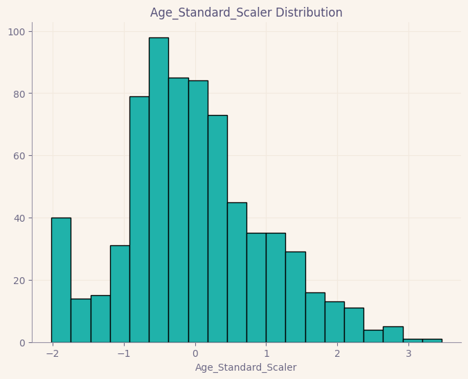
count    7.140000e+02
mean     2.388379e-16
std      1.000701e+00
min     -2.016979e+00
5%      -1.770360e+00
10%     -1.081480e+00
20%     -7.370406e-01
30%     -5.303766e-01
40%     -3.237127e-01
50%     -1.170488e-01
60%      1.447255e-01
70%      4.340550e-01
80%      7.784949e-01
90%      1.398487e+00
95%      1.811815e+00
99%      2.491739e+00
max      3.465126e+00
Name: Age_Standard_Scaler, dtype: float64

--------------------------------------------------

Summary for Age_Robuts_Scaler:

count    714.000000
mean       0.095056
std        0.812671
min       -1.542937
5%        -1.342657
10%       -0.783217
20%       -0.503497
30%       -0.335664
40%       -0.167832
50%        0.000000
60%        0.212587
70%        0.447552
80%        0.727273
90%        1.230769
95%        1.566434
99%        2.118601
max        2.909091
Name: Age_Robuts_Scaler, dtype: float64

--------------------------------------------------

Summary for Age_Min_Max_Scaler:

count    714.000000
mean       0.367921
std        0.182540
min        0.000000
5%         0.044986
10%        0.170646
20%        0.233476
30%        0.271174
40%        0.308872
50%        0.346569
60%        0.394320
70%        0.447097
80%        0.509927
90%        0.623021
95%        0.698417
99%        0.822443
max        1.000000
Name: Age_Min_Max_Scaler, dtype: float64

--------------------------------------------------
🗨️ Comment:
- 数值到分类(分箱)转换用于将数值变量转换为分类变量。例如,年龄变量被分为四分位数,并转换为分类变量。这可以用于以更有意义的方式对数据进行分组或建模。
titanic["Age_qcut"] = pd.qcut(titanic['Age'], 5)
titanic.head()
| PassengerId | Survived | Pclass | Name | Sex | Age | SibSp | Parch | Ticket | Fare | Cabin | Embarked | Age_Standard_Scaler | Age_Robuts_Scaler | Age_Min_Max_Scaler | Age_qcut | |
|---|---|---|---|---|---|---|---|---|---|---|---|---|---|---|---|---|
| 0 | 1 | 0 | 3 | Braund, Mr. Owen Harris | male | 22.0 | 1 | 0 | A/5 21171 | 7.2500 | NaN | S | -0.530377 | -0.335664 | 0.271174 | (19.0, 25.0] |
| 1 | 2 | 1 | 1 | Cumings, Mrs. John Bradley (Florence Briggs Th... | female | 38.0 | 1 | 0 | PC 17599 | 71.2833 | C85 | C | 0.571831 | 0.559441 | 0.472229 | (31.8, 41.0] |
| 2 | 3 | 1 | 3 | Heikkinen, Miss. Laina | female | 26.0 | 0 | 0 | STON/O2. 3101282 | 7.9250 | NaN | S | -0.254825 | -0.111888 | 0.321438 | (25.0, 31.8] |
| 3 | 4 | 1 | 1 | Futrelle, Mrs. Jacques Heath (Lily May Peel) | female | 35.0 | 1 | 0 | 113803 | 53.1000 | C123 | S | 0.365167 | 0.391608 | 0.434531 | (31.8, 41.0] |
| 4 | 5 | 0 | 3 | Allen, Mr. William Henry | male | 35.0 | 0 | 0 | 373450 | 8.0500 | NaN | S | 0.365167 | 0.391608 | 0.434531 | (31.8, 41.0] |
🔍Feature Extraction🔎
✨Binary Features: Flag, Bool, True-False✨
titanic = titanic_.copy()
titanic["Cabin_Bool"] = titanic["Cabin"].notnull().astype('int')
titanic.head()

# NaN values were converted to 0, and the rest were set to 1.
| PassengerId | Survived | Pclass | Name | Sex | Age | SibSp | Parch | Ticket | Fare | Cabin | Embarked | Cabin_Bool | |
|---|---|---|---|---|---|---|---|---|---|---|---|---|---|
| 0 | 1 | 0 | 3 | Braund, Mr. Owen Harris | male | 22.0 | 1 | 0 | A/5 21171 | 7.2500 | NaN | S | 0 |
| 1 | 2 | 1 | 1 | Cumings, Mrs. John Bradley (Florence Briggs Th... | female | 38.0 | 1 | 0 | PC 17599 | 71.2833 | C85 | C | 1 |
| 2 | 3 | 1 | 3 | Heikkinen, Miss. Laina | female | 26.0 | 0 | 0 | STON/O2. 3101282 | 7.9250 | NaN | S | 0 |
| 3 | 4 | 1 | 1 | Futrelle, Mrs. Jacques Heath (Lily May Peel) | female | 35.0 | 1 | 0 | 113803 | 53.1000 | C123 | S | 1 |
| 4 | 5 | 0 | 3 | Allen, Mr. William Henry | male | 35.0 | 0 | 0 | 373450 | 8.0500 | NaN | S | 0 |
titanic.groupby("Cabin_Bool").agg({"Survived": "mean"})
| Survived | |
|---|---|
| Cabin_Bool | |
| 0 | 0.299854 |
| 1 | 0.666667 |
🗨️ Comment:
- 我们需要统计地检验这个新创建的变量与因变量之间的关系。这可能是一个随机发生的情况,所以我们需要证明它。
from statsmodels.stats.proportion import proportions_ztest

test_stat, pvalue = proportions_ztest(count=[titanic.loc[titanic["Cabin_Bool"] == 1, "Survived"].sum(),
                                             titanic.loc[titanic["Cabin_Bool"] == 0, "Survived"].sum()],

                                      nobs=[titanic.loc[titanic["Cabin_Bool"] == 1, "Survived"].shape[0],
                                            titanic.loc[titanic["Cabin_Bool"] == 0, "Survived"].shape[0]])

print('Test Stat = %.4f, p-value = %.4f' % (test_stat, pvalue))
Test Stat = 9.4597, p-value = 0.0000
🗨️ Comment:
- 我们的测试是p1和p2的比例之间是否存在差异。
- p1和p2表示有和没有船舱号码的人的生存率。
- 由于p值小于0.05,H0被拒绝。
- p1和p2之间存在统计学上的显著差异。
titanic.loc[((titanic['SibSp'] + titanic['Parch']) > 0), "NEW_IS_ALONE"] = "NO"
titanic.loc[((titanic['SibSp'] + titanic['Parch']) == 0), "NEW_IS_ALONE"] = "YES"
titanic.groupby("NEW_IS_ALONE").agg({"Survived": "mean"})
| Survived | |
|---|---|
| NEW_IS_ALONE | |
| NO | 0.505650 |
| YES | 0.303538 |
🗨️ Comment:
- NO:有家人的人,YES:独自一人
- 看起来有家人的人的生存率更高。然而,我们需要统计地证明这一点,因为这可能是偶然发生的或由于多变量效应。
test_stat, pvalue = proportions_ztest(count=[titanic.loc[titanic["NEW_IS_ALONE"] == "YES", "Survived"].sum(),
                                             titanic.loc[titanic["NEW_IS_ALONE"] == "NO", "Survived"].sum()],

                                      nobs=[titanic.loc[titanic["NEW_IS_ALONE"] == "YES", "Survived"].shape[0],
                                            titanic.loc[titanic["NEW_IS_ALONE"] == "NO", "Survived"].shape[0]])

print('Test Stat = %.4f, p-value = %.4f' % (test_stat, pvalue))
Test Stat = -6.0704, p-value = 0.0000
🗨️ Comment:
- 由于p值小于0.05,H0被拒绝。
- 这个变量可能有重要影响。
✨Text Features✨
titanic = titanic_.copy()
# Letter count;

titanic["New_Name_Count"] = titanic["Name"].str.len()
# Word count;

titanic["New_Name_Word_Count"] = titanic["Name"].apply(lambda x: len(str(x).split(" ")))
# Catching Special Words;

titanic["New_Special"] = titanic["Name"].apply(lambda x: len([x for x in x.split() if x.startswith("Dr")]))

titanic.groupby("New_Special").agg({"Survived": ["mean","count"]})
| Survived | ||
|---|---|---|
| mean | count | |
| New_Special | ||
| 0 | 0.38252 | 881 |
| 1 | 0.50000 | 10 |
🗨️ Comment:
- 在这一部分,我们尝试从现有变量中派生新变量。
- 从包含姓名的变量中,我们可以确定姓名的长度、单词的数量,或者在姓名中具有特殊称号的个体的数量,并将这些值分配给新变量。
例如,有10个人的姓名中带有"Dr"。
✨Regex Features✨
titanic.head()
| PassengerId | Survived | Pclass | Name | Sex | Age | SibSp | Parch | Ticket | Fare | Cabin | Embarked | New_Name_Count | New_Name_Word_Count | New_Special | |
|---|---|---|---|---|---|---|---|---|---|---|---|---|---|---|---|
| 0 | 1 | 0 | 3 | Braund, Mr. Owen Harris | male | 22.0 | 1 | 0 | A/5 21171 | 7.2500 | NaN | S | 23 | 4 | 0 |
| 1 | 2 | 1 | 1 | Cumings, Mrs. John Bradley (Florence Briggs Th... | female | 38.0 | 1 | 0 | PC 17599 | 71.2833 | C85 | C | 51 | 7 | 0 |
| 2 | 3 | 1 | 3 | Heikkinen, Miss. Laina | female | 26.0 | 0 | 0 | STON/O2. 3101282 | 7.9250 | NaN | S | 22 | 3 | 0 |
| 3 | 4 | 1 | 1 | Futrelle, Mrs. Jacques Heath (Lily May Peel) | female | 35.0 | 1 | 0 | 113803 | 53.1000 | C123 | S | 44 | 7 | 0 |
| 4 | 5 | 0 | 3 | Allen, Mr. William Henry | male | 35.0 | 0 | 0 | 373450 | 8.0500 | NaN | S | 24 | 4 | 0 |
titanic['New_Title'] = titanic.Name.str.extract(' ([A-Za-z]+)\.', expand=False)
titanic[["New_Title", "Survived", "Age"]].groupby(["New_Title"]).agg({"Survived": "mean", "Age": ["count", "mean"]})
| Survived | Age | ||
|---|---|---|---|
| mean | count | mean | |
| New_Title | |||
| Capt | 0.000000 | 1 | 70.000000 |
| Col | 0.500000 | 2 | 58.000000 |
| Countess | 1.000000 | 1 | 33.000000 |
| Don | 0.000000 | 1 | 40.000000 |
| Dr | 0.428571 | 6 | 42.000000 |
| Jonkheer | 0.000000 | 1 | 38.000000 |
| Lady | 1.000000 | 1 | 48.000000 |
| Major | 0.500000 | 2 | 48.500000 |
| Master | 0.575000 | 36 | 4.574167 |
| Miss | 0.697802 | 146 | 21.773973 |
| Mlle | 1.000000 | 2 | 24.000000 |
| Mme | 1.000000 | 1 | 24.000000 |
| Mr | 0.156673 | 398 | 32.368090 |
| Mrs | 0.792000 | 108 | 35.898148 |
| Ms | 1.000000 | 1 | 28.000000 |
| Rev | 0.000000 | 6 | 43.166667 |
| Sir | 1.000000 | 1 | 49.000000 |
🗨️ Comment:
- 在这里,您可以观察到新创建的类别的频率和平均值,并进行推断。
✨Date Features✨
course = pd.read_csv("/kaggle/input/course-reviewsdataset/course_reviews.csv")
course.head()
| Rating | Timestamp | Enrolled | Progress | Questions Asked | Questions Answered | |
|---|---|---|---|---|---|---|
| 0 | 5.0 | 2021-02-05 07:45:55 | 2021-01-25 15:12:08 | 5.0 | 0.0 | 0.0 |
| 1 | 5.0 | 2021-02-04 21:05:32 | 2021-02-04 20:43:40 | 1.0 | 0.0 | 0.0 |
| 2 | 4.5 | 2021-02-04 20:34:03 | 2019-07-04 23:23:27 | 1.0 | 0.0 | 0.0 |
| 3 | 5.0 | 2021-02-04 16:56:28 | 2021-02-04 14:41:29 | 10.0 | 0.0 | 0.0 |
| 4 | 4.0 | 2021-02-04 15:00:24 | 2020-10-13 03:10:07 | 10.0 | 0.0 | 0.0 |
course.info()
<class 'pandas.core.frame.DataFrame'>
RangeIndex: 4323 entries, 0 to 4322
Data columns (total 6 columns):
 #   Column              Non-Null Count  Dtype
---  ------              --------------  -----
 0   Rating              4323 non-null   float64
 1   Timestamp           4323 non-null   object
 2   Enrolled            4323 non-null   object
 3   Progress            4323 non-null   float64
 4   Questions Asked     4323 non-null   float64
 5   Questions Answered  4323 non-null   float64
dtypes: float64(4), object(2)
memory usage: 202.8+ KB
course['Timestamp'] = pd.to_datetime(course["Timestamp"], format="%Y-%m-%d %H:%M:%S")
course['Year'] = course['Timestamp'].dt.year
course['Month'] = course['Timestamp'].dt.month
# The year difference between two dates;
course['Year_Diff'] = date.today().year - course['Timestamp'].dt.year
# The month difference between two dates;

course['Month_Diff'] = (date.today().year - course['Timestamp'].dt.year) * 12 + date.today().month - course['Timestamp'].dt.month
# Day names;

course['Day_Name'] = course['Timestamp'].dt.day_name()
course.head()
| Rating | Timestamp | Enrolled | Progress | Questions Asked | Questions Answered | Year | Month | Year_Diff | Month_Diff | Day_Name | |
|---|---|---|---|---|---|---|---|---|---|---|---|
| 0 | 5.0 | 2021-02-05 07:45:55 | 2021-01-25 15:12:08 | 5.0 | 0.0 | 0.0 | 2021 | 2 | 2 | 33 | Friday |
| 1 | 5.0 | 2021-02-04 21:05:32 | 2021-02-04 20:43:40 | 1.0 | 0.0 | 0.0 | 2021 | 2 | 2 | 33 | Thursday |
| 2 | 4.5 | 2021-02-04 20:34:03 | 2019-07-04 23:23:27 | 1.0 | 0.0 | 0.0 | 2021 | 2 | 2 | 33 | Thursday |
| 3 | 5.0 | 2021-02-04 16:56:28 | 2021-02-04 14:41:29 | 10.0 | 0.0 | 0.0 | 2021 | 2 | 2 | 33 | Thursday |
| 4 | 4.0 | 2021-02-04 15:00:24 | 2020-10-13 03:10:07 | 10.0 | 0.0 | 0.0 | 2021 | 2 | 2 | 33 | Thursday |
✨Feature Interaction✨
titanic = titanic_.copy()
titanic.head()
| PassengerId | Survived | Pclass | Name | Sex | Age | SibSp | Parch | Ticket | Fare | Cabin | Embarked | |
|---|---|---|---|---|---|---|---|---|---|---|---|---|
| 0 | 1 | 0 | 3 | Braund, Mr. Owen Harris | male | 22.0 | 1 | 0 | A/5 21171 | 7.2500 | NaN | S |
| 1 | 2 | 1 | 1 | Cumings, Mrs. John Bradley (Florence Briggs Th... | female | 38.0 | 1 | 0 | PC 17599 | 71.2833 | C85 | C |
| 2 | 3 | 1 | 3 | Heikkinen, Miss. Laina | female | 26.0 | 0 | 0 | STON/O2. 3101282 | 7.9250 | NaN | S |
| 3 | 4 | 1 | 1 | Futrelle, Mrs. Jacques Heath (Lily May Peel) | female | 35.0 | 1 | 0 | 113803 | 53.1000 | C123 | S |
| 4 | 5 | 0 | 3 | Allen, Mr. William Henry | male | 35.0 | 0 | 0 | 373450 | 8.0500 | NaN | S |
titanic["NEW_AGE_PCLASS"] = titanic["Age"] * titanic["Pclass"] # Age için stanartlaştırma işlemi gerekebilir.

titanic["NEW_FAMILY_SIZE"] = titanic["SibSp"] + titanic["Parch"] + 1

titanic.loc[(titanic['Sex'] == 'male') & (titanic['Age'] <= 21), 'NEW_SEX_CAT'] = 'youngmale'

titanic.loc[(titanic['Sex'] == 'male') & (titanic['Age'] > 21) & (titanic['Age'] < 50), 'NEW_SEX_CAT'] = 'maturemale'

titanic.loc[(titanic['Sex'] == 'male') & (titanic['Age'] >= 50), 'NEW_SEX_CAT'] = 'seniormale'

titanic.loc[(titanic['Sex'] == 'female') & (titanic['Age'] <= 21), 'NEW_SEX_CAT'] = 'youngfemale'

titanic.loc[(titanic['Sex'] == 'female') & (titanic['Age'] > 21) & (titanic['Age'] < 50), 'NEW_SEX_CAT'] = 'maturefemale'

titanic.loc[(titanic['Sex'] == 'female') & (titanic['Age'] >= 50), 'NEW_SEX_CAT'] = 'seniorfemale'
titanic.head()
| PassengerId | Survived | Pclass | Name | Sex | Age | SibSp | Parch | Ticket | Fare | Cabin | Embarked | NEW_AGE_PCLASS | NEW_FAMILY_SIZE | NEW_SEX_CAT | |
|---|---|---|---|---|---|---|---|---|---|---|---|---|---|---|---|
| 0 | 1 | 0 | 3 | Braund, Mr. Owen Harris | male | 22.0 | 1 | 0 | A/5 21171 | 7.2500 | NaN | S | 66.0 | 2 | maturemale |
| 1 | 2 | 1 | 1 | Cumings, Mrs. John Bradley (Florence Briggs Th... | female | 38.0 | 1 | 0 | PC 17599 | 71.2833 | C85 | C | 38.0 | 2 | maturefemale |
| 2 | 3 | 1 | 3 | Heikkinen, Miss. Laina | female | 26.0 | 0 | 0 | STON/O2. 3101282 | 7.9250 | NaN | S | 78.0 | 1 | maturefemale |
| 3 | 4 | 1 | 1 | Futrelle, Mrs. Jacques Heath (Lily May Peel) | female | 35.0 | 1 | 0 | 113803 | 53.1000 | C123 | S | 35.0 | 2 | maturefemale |
| 4 | 5 | 0 | 3 | Allen, Mr. William Henry | male | 35.0 | 0 | 0 | 373450 | 8.0500 | NaN | S | 105.0 | 1 | maturemale |
👻 Analysis Results:
特征工程是数据科学项目中至关重要的阶段,涵盖了一系列技术,使数据集更有意义和适合建模。在本节中,我们专注于异常值的检测和处理、处理缺失值、编码变量、特征缩放、提取新特征以及处理日期、文本和正则表达式特征等主题。
处理异常值对于清理数据集和提高模型性能至关重要。正确处理缺失值可以最大限度地减少数据损失,同时提高模型的可靠性。编码变量用于将分类数据转换为数值格式,可以提高模型性能。创建新特征可以为数据增加更多含义,并提升模型性能。最后,处理日期、文本和正则表达式可以处理更复杂的数据类型。
这些主题为数据工程师和数据科学家提供了组织数据集和增强建模能力的基本工具。特征工程是通过更好地理解数据集和提高建模能力来获得更好结果的关键步骤。


 2396
2396

 被折叠的 条评论
为什么被折叠?
被折叠的 条评论
为什么被折叠?
 到【灌水乐园】发言


