[论文阅读笔记16]BoT-SORT论文公式推导与代码解读

---

论文地址: BoT-SORT: Robust Associations Multi-Pedestrian Tracking
和OCSORT(解读见OCSORT)一样, 都是对Kalman滤波进行的改进. OCSORT是针对观测(检测器)不可靠时Kalman预测方差变大的问题, 对轨迹做了平滑. 而BoT-SORT是针对相机运动的问题, 加入了相机运动补偿. 也就是除了利用Kalman预测目标的新位置之外, 还利用稀疏光流(也就是提取目标之外的画面中的关键点, 来获得两帧之间画面的移动, 进而补偿Kalman得到的结果)

---

1. Kalman滤波

Kalman滤波遵循如下的更新步骤和预测步骤:

预测步:
$$\begin{gathered} {\hat{x}}_{t|t-1}=F_t{\hat{x}}_{t-1|t-1}+B_t{u}_t \\ {P}_{t|t-1}=F_t{P}_{t-1|t-1}{F}_t+Q \end{gathered}$$

更新步:
$$\begin{gathered} {\hat{x}}_{t|t}={\hat{x}}_{t|t-1}+K_t(z_t-H_t{\hat{x}}_{t|t-1}) \\ {K}_t=\frac{P_{t|t-1}{H}_t^T}{H_t^T{P}_{t|t-1}{H}_t+R_t} \\ {P}_{t|t}=P_{t|t-1}-K_t{H}_t{P}_{t|t-1} \end{gathered}$$

其中$Q$, $R$分别为输入(观测)和状态的噪声的协方差矩阵.

2. 状态变量的选择

在SORT中, 状态变量为[中心点, 面积, 高宽比, 速度, 面积变化率], 即$x=[x_c,y_c,a,s,\dot{x_c},\dot{y_c},\dot{s}]$, 从DeepSORT以后, 状态变量基本采用的是$x=[x_c,y_c,a,h,\dot{x_c},\dot{y_c},\dot{a},\dot{h}]$.

在BoT-SORT中, 作者简单地将状态变量改成了xywh及其导数, 即:$x=[x_c,y_c,w,h,\dot{x_c},\dot{y_c},\dot{w},\dot{h}]$, 类似地, 观测器的输入变量为$z=[z_{xc},z_{yc},z_w,z_h]$.

论文(1)(2)式

论文(3)(4)式, 关于噪声协方差矩阵的定义暂时没看懂, 看懂后补充

从消融实验的结果看, 按照这种方式更改状态变量MOTA, IDF1和HOTA指标大约有0.1 0.2左右的提升

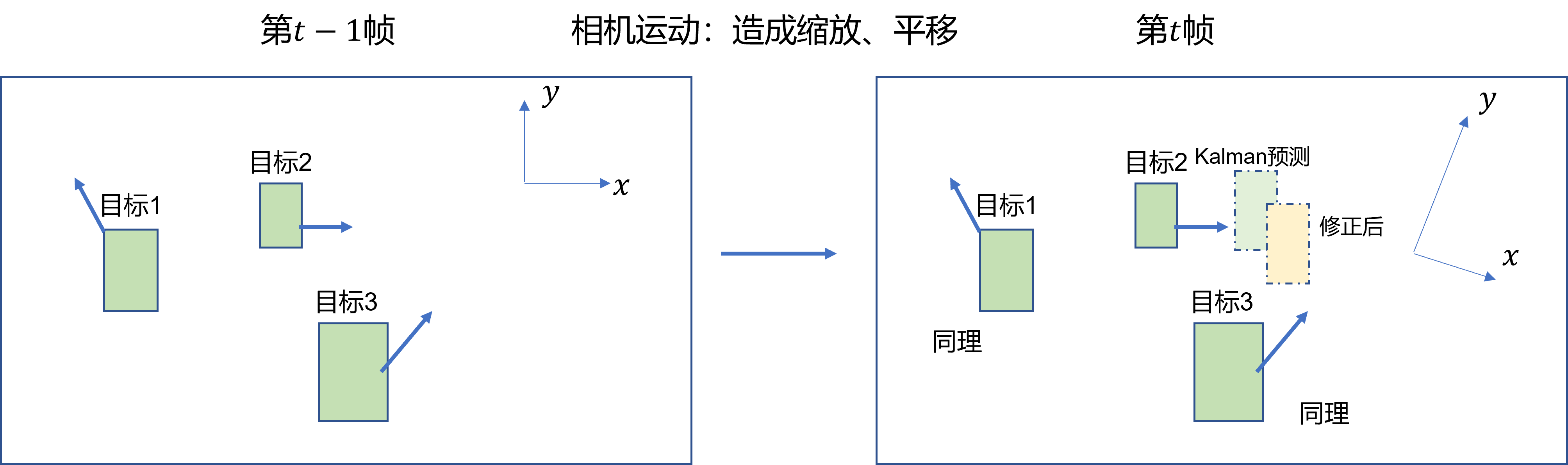
3. 相机运动补偿

这是BoT-SORT提出的核心思想.

由于相机运动, 可能会造成匹配的不准确. 然而我们缺乏相机运动的先验信息(例如导航等), 因此, 相邻两帧之间的图像配准(image registration)可以近似相机运动在图像二维平面上的投影.

这里可以理解为, 相机运动等同于坐标系的变换, 因此目标的位置, 运动方向等我们需要重新投影到新坐标系中, 因此我们需要求解坐标系的变换矩阵. 如下图所示:

因此, 利用 RANSAC算法得到平面坐标变化的仿射矩阵, 描述2维平面旋转变化矩阵为$M\in {\mathbb{R}}^{2\times 2}$, 平移变化向量为$T\in {\mathbb{R}}^2$, 定义仿射矩阵
$$A=[MT]\in {\mathbb{R}}^{2\times 3}$$

论文(5)式

假定Kalman预测后的结果为${\hat{x}}_{t|t-1}=[x_c,y_c,w,h,\dot{x_c},\dot{y_c},\dot{w},\dot{h}{]}^T$, 我们需要对中心点和高宽都应用仿射变换, 为了用一次矩阵乘法实现, 构造:

M k ∣ k − 1 ′ = d i a g { M , M , M , M } ∈ R 8 × 8 T k ∣ k − 1 ′ = [ T , 0 , 0 , 0 , 0 , 0 , 0 ] ∈ R 8 M'_{k|k-1}=diag\{M, M, M, M\}\in\mathbb{R}^{8\times 8}\\ T'_{k|k-1}=[T ,0, 0, 0, 0, 0, 0]\in\mathbb{R}^{8} Mk∣k−1′​=diag{M,M,M,M}∈R8×8Tk∣k−1′​=[T,0,0,0,0,0,0]∈R8

因此:

$${\hat{x}}_{t|t-1}^{\prime }=M_{k|k-1}^{\prime }{\hat{x}}_{t|t-1}+T_{k|k-1}^{\prime }$$

${\hat{x}}_{t|t-1}$的协方差矩阵变为(随机变量应用线性变换, 方差为系数平方关系):
$$P_{t|t-1}^{\prime }=M_{k|k-1}^{\prime }{P}_{t|t-1}{M}_{k|k-1}^{{}^{\prime }T}$$

论文(5)~(8)式

随后利用修正后的${\hat{x}}_{t|t-1}^{\prime }$和$P_{t|t-1}^{\prime }$再进行更新步.

论文(9)式

在实现中, 我们将画面中的目标扣去, 在其余的部分检测关键点, 来计算仿射矩阵:(tracker\gmc.py line120)

		# find the keypoints
        mask = np.zeros_like(frame)
        # mask[int(0.05 * height): int(0.95 * height), int(0.05 * width): int(0.95 * width)] = 255
        mask[int(0.02 * height): int(0.98 * height), int(0.02 * width): int(0.98 * width)] = 255
        if detections is not None:
            for det in detections:
                tlbr = (det[:4] / self.downscale).astype(np.int_)
                mask[tlbr[1]:tlbr[3], tlbr[0]:tlbr[2]] = 0

        keypoints = self.detector.detect(frame, mask)

        # compute the descriptors
        keypoints, descriptors = self.extractor.compute(frame, keypoints)

随后将相邻两帧的关键点进行匹配

		# Match descriptors.
        knnMatches = self.matcher.knnMatch(self.prevDescriptors, descriptors, 2)

如果关键点的个数足够, 就计算仿射矩阵

		 # Find rigid matrix
        if (np.size(prevPoints, 0) > 4) and (np.size(prevPoints, 0) == np.size(prevPoints, 0)):
            H, inliesrs = cv2.estimateAffinePartial2D(prevPoints, currPoints, cv2.RANSAC)

以上部分依赖于cv2库. 得到仿射矩阵后, 修正Kalman的结果(tracker\bot_sort.py line68):

def multi_gmc(stracks, H=np.eye(2, 3)):
        if len(stracks) > 0:
            multi_mean = np.asarray([st.mean.copy() for st in stracks])
            multi_covariance = np.asarray([st.covariance for st in stracks])

            R = H[:2, :2]
            R8x8 = np.kron(np.eye(4, dtype=float), R)
            t = H[:2, 2]

            for i, (mean, cov) in enumerate(zip(multi_mean, multi_covariance)):
                mean = R8x8.dot(mean)
                mean[:2] += t
                cov = R8x8.dot(cov).dot(R8x8.transpose())

                stracks[i].mean = mean
                stracks[i].covariance = cov

4. 匹配策略

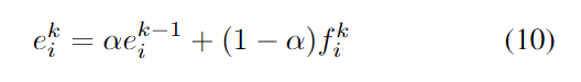
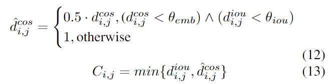
在匹配过程中, 利用指数滑动平均来平衡过去和当前的外观特征, 随后将运动特征和外观特征线性组合作为cost matrix, 如下两式所示:

对于外观和IoU都相似的目标, 给予更小的cost, 否则设为1, 并以此更新C中的元素:

最终结果如下表所示: