（ICLR-2022）关于局部注意力和动态深度卷积之间的联系(附录)

APPENDIX

A RELATION GRAPH

---

在图 3 中给出了一个关系图来描述卷积、depth-wise separable convolution（depth-wise convolution + $1\times 1$ convolution）、Vision Transformer、Local Vision Transformer 以及多层感知器（MLP）、Separable MLP 之间的关系在稀疏连接、权重共享和动态权重方面。表 7

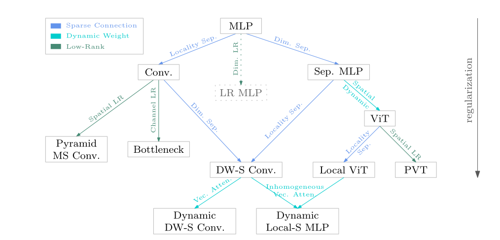
图 3：卷积 (Conv)、深度可分离卷积 (DW-S Conv)、Vision Transformer (ViT) 构建块、局部 ViT 构建块、Sep MLP（例如 MLP-Mixer 和 ResMLP）、动态深度的关系图在稀疏连通性和动态权重方面，可分离卷积（Dynamic DW-S Conv），以及动态局部可分离 MLP。 Dim = 包括空间和通道的维度，Sep = 可分离，LR = 低秩，MS Conv = 多尺度卷积，PVT = 金字塔视觉Transformer。

表 7：注意力、局部 MLP（局部注意力的非动态版本，注意力权重作为静态模型参数学习）、局部注意力、卷积、深度卷积（DW-Conv.）和动态变体（ D-DW-Conv.），以及在稀疏连接、权重共享和动态权重模式方面的 MLP 和 MLP 变体。 Spatial-mixing MLP（channel-separable MLP）对应于token-mixer MLP。 ‡$1\times 1$转化率也称为逐点（空间可分离）MLP。 权重可能在每组通道内共享。有关连接模式的说明，请参阅图 1。

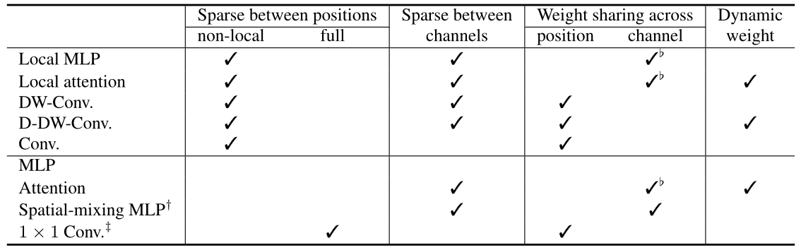
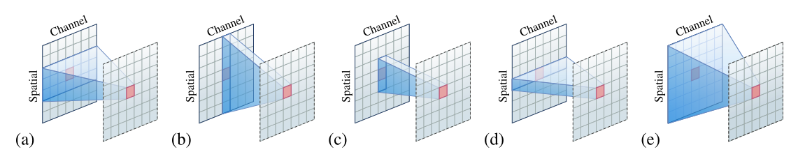
图 1：(a) 卷积、(b) 全局注意力和空间混合 MLP、© 局部注意力和深度卷积、(d) 逐点 MLP 或$1\times 1$卷积 (e) MLP（全连接层）。在空间维度上，为了清楚起见，使用一维来说明局部连接模式。

多层感知器 (MLP) 是一个全连接层：一层中的每个神经元（每个位置和每个通道的一个元素）都与前一层中的所有神经元相连。卷积和可分离 MLP 是 MLP 的稀疏版本。连接权重可以表示为张量（例如，3D 张量，空间的二维和通道的一维），并且张量的低秩近似可用于正则化 MLP。

卷积是一个局部连接层，通过将每个神经元连接到一个小的局部窗口中的神经元而形成，其权重在空间位置之间共享。 Depth-wise separable convolution是通过将卷积分解成两个分量形成的：一个是point-wise $1\times 1$卷积，将信息跨通道混合，另一个是depth-wise convolution，混合空间信息。卷积的其他变体，例如瓶颈、多尺度卷积或金字塔，可以被视为低秩变体。

可分离 MLP（例如 MLP-Mixer 和 ResMLP）将 3D 张量重塑为具有空间维度和通道维度的 2D 格式。可分离 MLP 由两个分别沿两个维度的稀疏 MLP 组成，它们是通过将输入神经元分成组而形成的。关于通道稀疏性，同一通道中的神经元组成一个组，对每组进行一次 MLP，MLP 参数在组间共享，形成第一个稀疏 MLP（空间/token混合）。通过将同一位置的神经元观察到一组来完成类似的过程，形成第二个稀疏 MLP（通道混合）。

Vision Transformer 是可分离 MLP 的动态版本。第一个稀疏 MLP（空间/token混合）中的权重是从每个实例动态预测的。 Local Vision Transformer 是 Vision Transformer 的空间稀疏版本：每个输出神经元都连接到局部窗口中的输入神经元。 PVT是 Vision Transformer 的金字塔（空间采样/低秩）变体。

深度可分离卷积也可以被视为可分离 MLP 的空间稀疏版本。在第一个稀疏 MLP（空间/token混合）中，每个输出神经元仅依赖于局部窗口中的输入神经元，形成深度卷积。此外，连接权重是跨空间位置共享的，而不是跨通道共享的。

B MATRIX FORM EXPLANATION

---

使用矩阵形式来解释各个层的稀疏连通性以及它们是如何通过修改 MLP 获得的。

MLP。术语MLP，即多层感知器，在任何前馈神经网络中都使用得很模糊，有时使用得很松散。采用其中一种常见的定义，并使用它来指代全连接层。讨论基于一个全连接的层，可以很容易地推广到两个或更多全连接的层。除非线性单位和其他单位外，一个主要组成部分是线性变换：
$$\mathbf{y}=\mathbf{W}\mathbf{x}(9)$$
其中$\mathbf{x}$表示输入神经元，$\mathbf{y}$表示输出神经元，$\mathbf{W}$表示连接权重，例如$\mathbf{W}\in {\mathbb{R}}^{NC\times NC}$，其中$N$是位置数，$C$是通道数。

卷积。考虑单通道的1D情况（2D情况类似），连接权重矩阵$\mathbf{W}\in {\mathbb{R}}^{N\times N}$为以下稀疏形式，也称为Toeplitz矩阵（以窗口大小3为例）：
$$\mathbf{W}=\left[\begin{array}{ccccccc}{a}_2& a_3& 0& 0& \cdots & 0& a_1\\ a_1& a_2& a_3& 0& \cdots & 0& 0\\ ⋮& ⋮& ⋮& ⋮& \ddots & ⋮& ⋮\\ a_3& 0& 0& 0& \cdots & a_1& a_2\end{array}\right](10)$$
对于$C$通道的情况，按通道将输入组织成一个向量通道：${\left[\begin{array}{llll}{\mathbf{x}}_1^{\top }& {\mathbf{x}}_2^{\top }& \dots & {\mathbf{x}}_C^{\top }\end{array}\right]}^{\top }$，因此对于$c_o$输出通道，逐通道连接权重矩阵${\mathbf{W}}_{c_o}=\left[{\mathbf{W}}_{c_{o}1}{\mathbf{W}}_{c_{o}2}\dots {\mathbf{W}}_{c_{o}C}\right]$（${\mathbf{W}}_{c_{o}i}$的形式与上式相同）。整个表格可以写成
$$\left[\begin{array}{c}{\mathbf{y}}_1\\ {\mathbf{y}}_2\\ ⋮\\ {\mathbf{y}}_C\end{array}\right]=\left[\begin{array}{c}{\mathbf{W}}_1\\ {\mathbf{W}}_2\\ ⋮\\ {\mathbf{W}}_C\end{array}\right]\left[\begin{array}{c}{\mathbf{x}}_1\\ {\mathbf{x}}_2\\ ⋮\\ {\mathbf{x}}_C\end{array}\right]$$

Sep. MLP 。 Sep. MLP，例如 ResMLP 和 MLP-Mixer，由两种块稀疏矩阵组成：一种用于通道混合，另一种用于空间混合。在输入按通道组织的情况下（每个通道中的神经元形成一个组），$\mathbf{x}={\left[{\mathbf{x}}_1^{\top }{\mathbf{x}}_2^{\top }\cdots {\mathbf{x}}_C^{\top }\right]}^{\top }$，连接权重矩阵为块稀疏形式：
$$\mathbf{W}=\left[\begin{array}{ccccc}{\mathbf{W}}_c& 0& \cdots & 0& 0\\ 0& {\mathbf{W}}_c& \cdots & 0& 0\\ ⋮& ⋮& \ddots & ⋮& ⋮\\ 0& 0& \cdots & 0& {\mathbf{W}}_c\end{array}\right]$$
其中块矩阵${\mathbf{W}}_c\in {\mathbb{R}}^{N\times N}$在所有通道之间共享，并且可以修改共享模式以在每组通道内共享权重。

输入可以逐个位置重塑（每个位置的神经元形成一个组）：$\mathbf{x}={\left[{\mathbf{x}}_1^{\top }{\mathbf{x}}_2^{\top }\cdots {\mathbf{x}}_C^{\top }\right]}^{\top }$，类似地，可以用块稀疏形式表示另外一个连接权重矩阵（它本质上是一个$1\times 1$卷积，${\mathbf{W}}_p\in {\mathbb{R}}^{C\times C}$）：
$${\mathbf{W}}^{\prime }=\left[\begin{array}{ccccc}{\mathbf{W}}_p& 0& \cdots & 0& 0\\ 0& {\mathbf{W}}_p& \cdots & 0& 0\\ ⋮& ⋮& \ddots & ⋮& ⋮\\ 0& 0& \cdots & 0& {\mathbf{W}}_p\end{array}\right]$$
在交错组卷积中研究了块稀疏性的形式，而没有在组之间共享权重。

Sep. MLP也可以看成是用Kronecker克积来逼近连接矩阵，
$$\mathbf{W}\mathbf{x}=\mathrm{vec}(\mathbf{A}\mathrm{mat}(\mathbf{x})\mathbf{B})$$

这里，$\mathbf{W}={\mathbf{B}}^{\top }\otimes \mathbf{A}={\mathbf{W}}_c^{\top }\otimes {\mathbf{W}}_p$。$\otimes$是Kronecker乘积算子。mat $(\mathbf{x})$将向量$\mathbf{x}$重塑为 2D 矩阵形式，而vec $(\mathbf{x})$将 2D 矩阵重塑为向量形式。在 Sep. MLP 中，2D 矩阵mat $(\mathbf{x})\in {\mathbb{R}}^{C\times N}$被组织成每一行对应一个通道，每一列对应一个空间位置。 CCNet和interlaced self-attention使用 Kronecker 积来逼近空间连接：前者沿 x 和 y 轴以 2D 矩阵形式重塑向量，而后者通过窗口重塑矢量窗口。

视觉Transformer (ViT)。矩阵形式类似于 Sep. MLP 。不同之处在于矩阵${\mathbf{W}}_c$是从每个图像实例中预测的。 ViT 中的权重预测方式有一个好处：处理任意数量的输入神经元。

深度可分离卷积。有两个基本组成部分：深度卷积和$1\times 1$卷积，与 Sep. MLP 中的通道混合 MLP 相同。深度卷积可以写成矩阵形式：
$$\left[\begin{array}{c}{\mathbf{y}}_1\\ {\mathbf{y}}_2\\ ⋮\\ {\mathbf{y}}_C\end{array}\right]=\left[\begin{array}{cccc}{\mathbf{W}}_{11}& 0& \cdots & 0\\ 0& {\mathbf{W}}_{22}& \cdots & 0\\ ⋮& ⋮& \ddots & ⋮\\ 0& 0& \cdots & {\mathbf{W}}_{CC}\end{array}\right]\left[\begin{array}{c}{\mathbf{x}}_1\\ {\mathbf{x}}_2\\ ⋮\\ {\mathbf{x}}_C\end{array}\right],$$
其中${\mathbf{W}}_{cc}$的形式与公式 10 相同。

局部 ViT。在非重叠窗口分区的情况下，局部 ViT 只是简单地在每个窗口上单独重复 ViT，线性投影应用于键、值和查询，在窗口之间共享。在重叠的情况下，形式有点复杂，但直觉是一样的。极端情况下，分区与卷积相同，形式如下：
$$\left[\begin{array}{c}{\mathbf{y}}_1\\ {\mathbf{y}}_2\\ ⋮\\ {\mathbf{y}}_C\end{array}\right]=\left[\begin{array}{cccc}{\mathbf{W}}^d& 0& \cdots & 0\\ 0& {\mathbf{W}}^d& \cdots & 0\\ ⋮& ⋮& \ddots & ⋮\\ 0& 0& \cdots & {\mathbf{W}}^d\end{array}\right]\left[\begin{array}{c}{\mathbf{x}}_1\\ {\mathbf{x}}_2\\ ⋮\\ {\mathbf{x}}_C\end{array}\right],$$
其中动态权重矩阵${\mathbf{W}}^d$如下所示：
$${\mathbf{W}}^d=\left[\begin{array}{ccccccc}{a}_{12}& a_{13}& 0& 0& \cdots & 0& a_{11}\\ a_{21}& a_{22}& a_{23}& 0& \cdots & 0& 0\\ ⋮& ⋮& ⋮& ⋮& \ddots & ⋮& ⋮\\ a_{N3}& 0& 0& 0& \cdots & a_{N1}& a_{N2}\end{array}\right].$$

低秩 MLP 。低秩 MLP 使用两个低秩矩阵的乘积来逼近等式 9 中的连接权重矩阵$\mathbf{W}\in {\mathbb{R}}^{D_o\times D_i}$：
$$\mathbf{W}\leftarrow {\mathbf{W}}_{D_{o}r}{\mathbf{W}}_{r{D}_i},$$
其中$r$是一个小于$D_i$和$D_o$的数。

金字塔。金字塔网络中的下采样过程可视为空间低秩：$\mathbf{W}\left(\in {\mathbb{R}}^{NC\times NC}\right)\to {\mathbf{W}}^{\prime }\left(\in {\mathbb{R}}^{N^{\prime }C\times N^{\prime }C}\right)$，其中在分辨率降低的情况下$N^{\prime }$等于$\frac{N}{4}$乘以$\frac{1}{2}$。如果输入和输出通道的数量不同，则变为$\mathbf{W}\left(\in {\mathbb{R}}^{N{C}^{\prime }\times NC}\right)\to {\mathbf{W}}^{\prime }\left(\in {\mathbb{R}}^{N^{\prime }{C}^{\prime }\times N^{\prime }C}\right)$。

多尺度并行卷积。 HRNet中使用的多尺度并行卷积也可以看作是空间低秩。考虑四个尺度的情况，多尺度并行卷积可以形成如下：
$$\mathbf{W}\to \left[\begin{array}{l}{\mathbf{W}}_1\in {\mathbb{R}}^{N{C}_1}\\ {\mathbf{W}}_2\in {\mathbb{R}}^{N{C}_2}\\ {\mathbf{W}}_3\in {\mathbb{R}}^{N{C}_3}\\ {\mathbf{W}}_4\in {\mathbb{R}}^{N{C}_4}\end{array}\right]\to \left[\begin{array}{c}{\mathbf{W}}_1^{\prime }\in {\mathbb{R}}^{N{C}_1}\\ {\mathbf{W}}_2^{\prime }\in {\mathbb{R}}^{\frac{N}{4}{C}_2}\\ {\mathbf{W}}_3^{\prime }\in {\mathbb{R}}^{\frac{N}{16}{C}_3}\\ {\mathbf{W}}_4^{\prime }\in {\mathbb{R}}^{\frac{N}{64}{C}_4}\end{array}\right],$$
其中$C_1,C_2,C_3$和$C_4$是四种分辨率的通道数。

C LOCAL ATTENTION VS CONVOLUTION: DYNAMIC WEIGHTS

---

以窗口大小为$2K+1$的一维情况为例来说明动态权重预测方式。令 { x i − K , … , x i , … , x i + k } \left\{\mathbf{x}_{i-K}, \ldots, \mathbf{x}_{i}, \ldots, \mathbf{x}_{i+k}\right\} {xi−K​,…,xi​,…,xi+k​}对应于第$i$个窗口中的$(2K+1)$个位置， { w i − K , … , w i , … , w i + K } \left\{w_{i-K}, \ldots, w_{i}, \ldots, w_{i+K}\right\} {wi−K​,…,wi​,…,wi+K​}是更新第$i$个（中心）位置表示的相应动态权重。可以很容易地扩展到每个位置的多个权重，例如 M-head attention 和更新其他位置的表示。

非均匀动态卷积。仅使用单个线性投影的情况来说明非均匀动态卷积。将讨论的属性对于更线性的投影是相似的。动态权重预测如下：
$$\left[\begin{array}{c}{w}_{i-K}\\ ⋮\\ w_i\\ ⋮\\ w_{i+K}\end{array}\right]=\Theta {\mathbf{x}}_i=\left[\begin{array}{c}{\theta }_{-K}^{\top }\\ ⋮\\ {\theta }_0^{\top }\\ ⋮\\ {\theta }_K^{\top }\end{array}\right]{\mathbf{x}}_i$$

可以看出，动态卷积通过不同位置的不同参数来学习每个位置的权重，例如${\theta }_k$对应$w_{i+k}$。它将窗口中的位置视为向量形式，保持空间顺序信息。

点积注意力。单头情况下的点积注意力机制预测权重如下：
$$\left[\begin{array}{c}{w}_{i-K}\\ ⋮\\ w_i\\ ⋮\\ w_{i+K}\end{array}\right]=\left[\begin{array}{c}{\left({\mathbf{x}}_{i-K}\right)}^{\top }\\ ⋮\\ {\left({\mathbf{x}}_i\right)}^{\top }\\ ⋮\\ {\left({\mathbf{x}}_{i+K}\right)}^{\top }\end{array}\right]{\mathbf{P}}_k^{\top }{\mathbf{P}}_q{\mathbf{x}}_i$$
点积注意力对所有位置使用相同的参数${\mathbf{P}}_k^{\top }{\mathbf{P}}_q$。权重取决于同一位置的特征，例如，$w_{i-k}$对应于${\mathbf{x}}_{i-k}$。它在某种意义上将窗口中的位置视为一种集合形式，丢失了空间顺序信息。

重写如下：
$${\Theta }_d=\left[\begin{array}{c}{\left({\mathbf{x}}_{i-K}\right)}^{\top }\\ ⋮\\ {\left({\mathbf{x}}_i\right)}^{\top }\\ ⋮\\ {\left({\mathbf{x}}_{i+K}\right)}^{\top }\end{array}\right]{\mathbf{P}}_k^{\top }\mathbf{P}$$
从中可以看到参数${\Theta }_d$是动态预测的。换句话说，点积注意力可以看作是一个两级的动态方案。

相对位置嵌入等效于添加保留空间顺序信息的静态权重：
$$\left[\begin{array}{c}{w}_{i-K}\\ ⋮\\ w_i\\ ⋮\\ w_{i+K}\end{array}\right]={\Theta }_d{\mathbf{x}}_i+\left[\begin{array}{c}{\beta }_{-K}\\ ⋮\\ {\beta }_0\\ ⋮\\ {\beta }_K\end{array}\right]（23）$$
一个简单的变体是静态$\Theta$和动态${\Theta }_d$的组合：
$$\left[\begin{array}{c}{w}_{i-K}\\ ⋮\\ w_i\\ ⋮\\ w_{i+K}\end{array}\right]=\left({\Theta }_d+\Theta \right)$$

卷积注意力。引入了卷积注意力框架，使其享受动态卷积和点积注意力的好处：保持空间顺序信息和两级动态权重预测。

卷积后注意力机制左乘一个矩阵（内核大小为 3）：
$${\Theta }_d=\left[\begin{array}{ccccccc}{a}_2& a_3& 0& 0& \cdots & 0& a_1\\ a_1& a_2& a_3& 0& \cdots & 0& 0\\ ⋮& ⋮& ⋮& ⋮& \ddots & ⋮& ⋮\\ a_3& 0& 0& 0& \cdots & a_1& a_2\end{array}\right]\left[\begin{array}{c}{\left({\mathbf{x}}_{i-K}\right)}^{\top }\\ ⋮\\ {\left({\mathbf{x}}_i\right)}^{\top }\\ ⋮\\ {\left({\mathbf{x}}_{i+K}\right)}^{\top }\end{array}\right]{\mathbf{P}}_k^{\top }{\mathbf{P}}_q$$
这可以看作是相对位置嵌入的一种变体（公式 23）。在左矩阵是对角矩阵的简化情况下，它可以看作是相对位置嵌入的乘积版本（公式 23 是一个加法版本）。

可以执行卷积核大小为 3，跨通道共享核权重（不共享权重也可以），然后进行点积注意力。这称为预卷积注意：对表示进行卷积。这两个过程可以写成如下（省略卷积后面的BN和ReLU），
$$\left[\begin{array}{c}{w}_{i-K}\\ ⋮\\ w_i\\ ⋮\\ w_{i+K}\end{array}\right]=\left[\begin{array}{ccccccc}{a}_1& a_2& a_3& \cdots & 0& 0& 0\\ 0& a_1& a_1& \cdots & 0& 0& 0\\ ⋮& ⋮& ⋮& \ddots & ⋮& ⋮& ⋮\\ 0& 0& 0& \cdots & a_2& a_3& 0\\ 0& 0& 0& \cdots & a_1& a_2& a_3\end{array}\right]\left[\begin{array}{c}{\left({\mathbf{x}}_{i-K-1}\right)}^{\top }\\ {\left({\mathbf{x}}_{i-K}\right)}^{\top }\\ ⋮\\ {\left({\mathbf{x}}_i\right)}^{\top }\\ ⋮\\ {\left({\mathbf{x}}_{i+K}\right)}^{\top }\\ {\left({\mathbf{x}}_{i+K+1}\right)}^{\top }\end{array}\right]{\mathbf{P}}_k^{\top }{\mathbf{P}}_q\left[{\mathbf{x}}_{i-1}{\mathbf{x}}_i{\mathbf{x}}_{i+1}\right]\left[\begin{array}{c}{a}_2\\ a_3\end{array}\right]$$
它可以推广到使用普通卷积：
$$\left[\begin{array}{c}{w}_{i-K}\\ ⋮\\ w_i\\ ⋮\\ w_{i+K}\end{array}\right]={\mathbf{C}}^{\prime }\left[\begin{array}{cccc}{\mathbf{x}}_{i-K-1}& {\mathbf{x}}_{i-K-1}& \cdots & {\mathbf{x}}_{i-K-1}\\ {\mathbf{x}}_{i-K}& {\mathbf{x}}_{i-K}& \cdots & {\mathbf{x}}_{i-K}\\ ⋮& ⋮& \ddots & ⋮\\ {\mathbf{x}}_i& {\mathbf{x}}_i& \cdots & {\mathbf{x}}_i\\ ⋮& ⋮& \ddots & ⋮\\ {\mathbf{x}}_{i+K}& {\mathbf{x}}_{i+K}& \cdots & {\mathbf{x}}_{i+K}\\ {\mathbf{x}}_{i+K+1}& {\mathbf{x}}_{i+K+1}& \cdots & {\mathbf{x}}_{i+K+1}\end{array}\right]{\mathbf{P}}_q{\mathbf{C}}_3\left[\begin{array}{c}{\mathbf{x}}_{i-1}\\ {\mathbf{x}}_i\\ {\mathbf{x}}_{i+1}\end{array}\right]$$
这里，${\mathbf{C}}^{\prime }$是一个$(2K+1)$行矩阵，可以很容易地从卷积核${\mathbf{C}}_3$推导出来。$(2K+1)$个权重 { w i − 1 , w i , w i + 1 } \left\{w_{i-1}, w_{i}, w_{i+1}\right\} {wi−1​,wi​,wi+1​}分别对应于$\mathbf{C}$中的$(2K+1)$行。这意味着这三个位置是有区别的，每个窗口中的相同位置对应于同一行。这解释了为什么在采用卷积时不需要位置嵌入。使用不同的对$\left({\mathbf{W}}_q,{\mathbf{W}}_k\right)$会导致每个位置有更多的权重，例如，M 对对应于 M-head attention。