基于注意力机制的Encoder-Decoder翻译器

https://tensorflow.google.cn/tutorials/text/nmt_with_attention

前言

将训练一个<西班牙语/英语>的sequence to sequence模型，模型中采用了Encoder-Decoder结构、注意力机制，训练过程中还使用了Teacher forcing的方法。
本文基于个人理解对代码和相关技术作相应介绍，如有错误欢迎评论指正

---

代码解析

1. Download and prepare the dataset 数据下载和预处理

语言翻译训练数据包可在线下载

# Converts the unicode file to ascii
def unicode_to_ascii(s):
  return ''.join(c for c in unicodedata.normalize('NFD', s)
      if unicodedata.category(c) != 'Mn')
      
def preprocess_sentence(w):
  w = unicode_to_ascii(w.lower().strip())
  # creating a space between a word and the punctuation following it
  # eg: "he is a boy." => "he is a boy ."
  # Reference:- https://stackoverflow.com/questions/3645931/python-padding-punctuation-with-white-spaces-keeping-punctuation
  w = re.sub(r"([?.!,¿])", r" \1 ", w)
  w = re.sub(r'[" "]+', " ", w)
  # replacing everything with space except (a-z, A-Z, ".", "?", "!", ",")
  w = re.sub(r"[^a-zA-Z?.!,¿]+", " ", w)
  w = w.strip()
  # adding a start and an end token to the sentence
  # so that the model know when to start and stop predicting.
  w = '<start> ' + w + ' <end>'
  return w

数据的预处理包括：

1. unicode 编码转ascii编码
2. 全小写字母化并去除首尾空格
3. 查找标点符号并在单词和标点符号之间插入空格以区分开
4. 仅保留语言中可能出现的符号和字母
   中文翻译可以添加 \u4e00-\u9fa5 汉字和中文标点符号
5. 添加首尾标记符号 <start> 和 <end>

---

# 1. Remove the accents
# 2. Clean the sentences
# 3. Return word pairs in the format: [ENGLISH, SPANISH]
def create_dataset(path, num_examples):
  lines = io.open(path, encoding='UTF-8').read().strip().split('\n')

  #word_pairs = [[preprocess_sentence(w) for w in l.split('\t')]  for l in lines[:num_examples]]
  word_pairs = [[preprocess_sentence(w) for w in l.split('\t')[:2]]  for l in lines[:num_examples]]

  return zip(*word_pairs)

原代码没有清理掉多余信息，因此取了每行前两个元素，即构建了以 [ENGLISH，SPANISH] 为pair的[target, input]数据集。

---

def tokenize(lang):
  lang_tokenizer = tf.keras.preprocessing.text.Tokenizer(
      filters='')
  lang_tokenizer.fit_on_texts(lang)

  tensor = lang_tokenizer.texts_to_sequences(lang)

  tensor = tf.keras.preprocessing.sequence.pad_sequences(tensor,
                                                         padding='post')

  return tensor, lang_tokenizer

def load_dataset(path, num_examples=None):
  # creating cleaned input, output pairs
  targ_lang, inp_lang = create_dataset(path, num_examples)

  input_tensor, inp_lang_tokenizer = tokenize(inp_lang)
  target_tensor, targ_lang_tokenizer = tokenize(targ_lang)

  return input_tensor, target_tensor, inp_lang_tokenizer, targ_lang_tokenizer

文本本身是无法交给神经网络进行训练的，因此我们需要将其映射成数字ID以便网络识别。
这里利用keras实现的Tokenizer类，流程如下：

1. 初始化Tokenizer，以空格过滤来识别每个单词
2. fit_on_texts(text)
   功能：建立文本词表
   参数texts ：要用以训练的文本列表
   返回值： 无
3. texts_to_sequences(texts)
   功能：将文本转换成对应的数字序列
   参数texts ：待转为序列的文本列表
   返回值： 序列的列表，列表中每个序列对应于一段输入文本
4. pad_sequences(sequence, padding=‘post’)
   功能：将数字序列填充成相同长度
   参数padding ：‘pre’ 前补0，'post’后补0
   参数sequence：待填充的序列
   参数maxlen=None：默认填充至列表中最大长度的序列
   返回值： 填充后的序列的列表

---

#Try experimenting with the size of that dataset
num_examples = 30000
input_tensor, target_tensor, inp_lang, targ_lang = load_dataset(path_to_file, num_examples)
input_tensor_train, input_tensor_val, target_tensor_train, target_tensor_val = train_test_split(input_tensor, target_tensor, test_size=0.2)
#Create a tf.data dataset
BUFFER_SIZE = len(input_tensor_train)
BATCH_SIZE = 64
steps_per_epoch = len(input_tensor_train)//BATCH_SIZE
embedding_dim = 256
units = 1024
vocab_inp_size = len(inp_lang.word_index)+1
vocab_tar_size = len(targ_lang.word_index)+1

dataset = tf.data.Dataset.from_tensor_slices((input_tensor_train, target_tensor_train)).shuffle(BUFFER_SIZE)
dataset = dataset.batch(BATCH_SIZE, drop_remainder=True)

• 按8:1的比例划分训练集和验证集
• 配置相关参数，生成数据集

---

2. Write the encoder and decoder model 构建编码器和解码器模型

实现了一个带有注意力机制的编码器-解码器模型，注意力机制详见后文。

Encoder model 编码器模型

class Encoder(tf.keras.Model):
  def __init__(self, vocab_size, embedding_dim, enc_units, batch_sz):
    super(Encoder, self).__init__()
    self.batch_sz = batch_sz
    self.enc_units = enc_units
    self.embedding = tf.keras.layers.Embedding(vocab_size, embedding_dim)
    self.gru = tf.keras.layers.GRU(self.enc_units,
                                   return_sequences=True,
                                   return_state=True,
                                   recurrent_initializer='glorot_uniform')

  def call(self, x, hidden):
    x = self.embedding(x)
    output, state = self.gru(x, initial_state = hidden)
    return output, state

  def initialize_hidden_state(self):
    return tf.zeros((self.batch_sz, self.enc_units))

• Embedding layer 嵌入层
• GRU 循环神经网络层
  • return_sequences=True, 输出shape为(batch_size, sequence_length, units)的编码器输出(enc_output)
  • return_state=True, 输出shape为(batch_size, units)的编码器隐藏层状态(enc_hidden)

主要用于将输入的vocab序列通过Embedding 和 GRU进行编码输出，得到enc_output和对应的enc_state，后续将被重复利用以尽可能的利用输入信息。

---

Attention layer ( BahdanauAttention) 注意力层（以Bahdanau style为例）

class BahdanauAttention(tf.keras.layers.Layer):
  def __init__(self, units):
    super(BahdanauAttention, self).__init__()
    self.W1 = tf.keras.layers.Dense(units)
    self.W2 = tf.keras.layers.Dense(units)
    self.V = tf.keras.layers.Dense(1)

  def call(self, query, values):
    # query hidden state shape == (batch_size, hidden size)
    # query_with_time_axis shape == (batch_size, 1, hidden size)
    # values shape == (batch_size, sequence_len, hidden size)
    # we are doing this to broadcast addition along the time axis to calculate the score
    query_with_time_axis = tf.expand_dims(query, 1)

    # score shape == (batch_size, sequence_length, 1)
    # we get 1 at the last axis because we are applying score to self.V
    # the shape of the tensor before applying self.V is (batch_size, max_length, units)
    score = self.V(tf.nn.tanh(
        self.W1(query_with_time_axis) + self.W2(values)))

    # attention_weights shape == (batch_size, sequence_length, 1)
    attention_weights = tf.nn.softmax(score, axis=1)

    # context_vector shape after sum == (batch_size, hidden_size)
    context_vector = attention_weights * values
    context_vector = tf.reduce_sum(context_vector, axis=1)

    return context_vector, attention_weights

Decoder的组成层之一，初始化后每次调用的参数为解码器隐藏层状态(dec_hidden)(对应query)和编码器输出(enc_output)（对应value）

• 相同尺寸的全连接层 W1 和 W2，用于抽象并求和 dec_hidden 信息和 enc_output 信息。
  dec_hidden 初始赋值为编码器隐藏层状态(enc_hidden)

• 尺寸为1的全连接层V，用于获得分数(score) 并计算 注意力权重(attention_weights), shape皆为(batch_size, sequence_length, 1)，最后与enc_output相乘并在axis=1维度上求和降维，得到上下文向量(context_vector)。计算过程公式如下图所示。
  

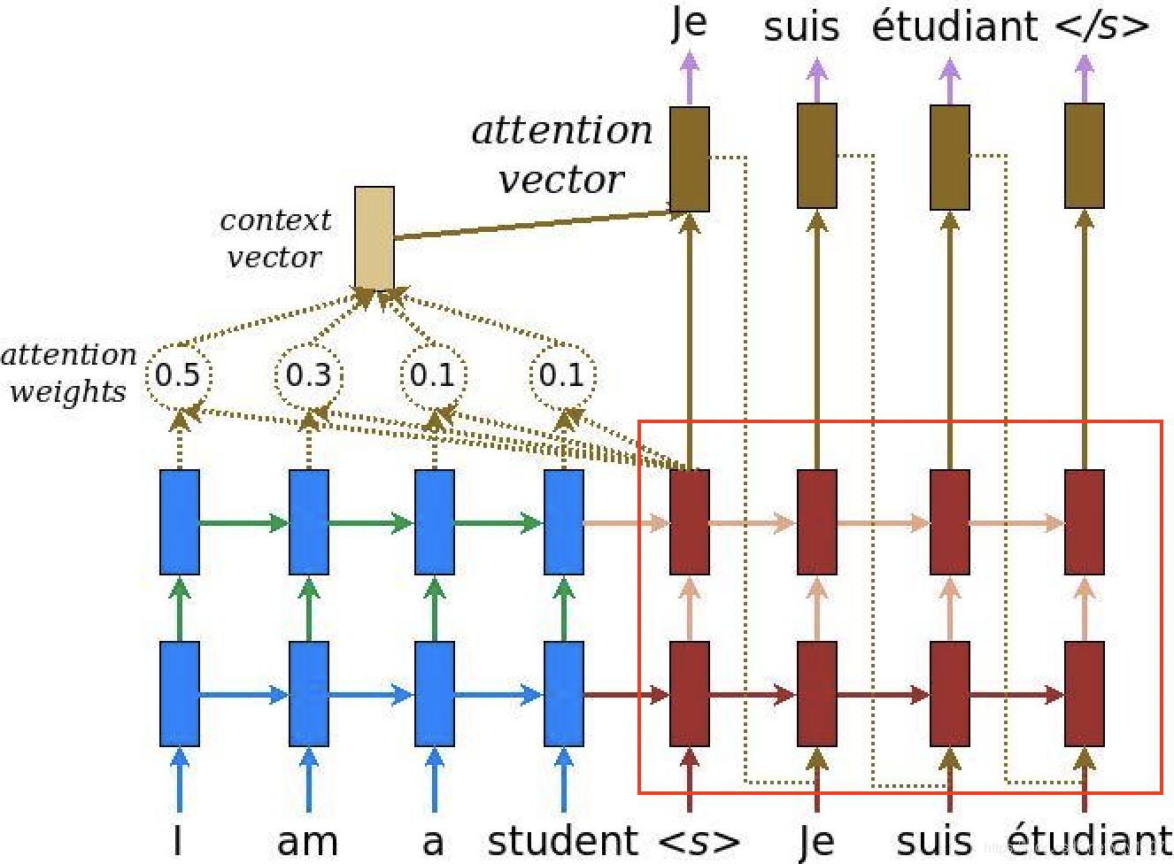
  • ${\alpha }_{ts}$ ：注意力权重(attention_weights)，表征第s个input_word对当前时刻t的应输出的target word的影响力。一般情况是，与应输出单词完全对应位置的输入单词权重最大，其前一个和后一个的权重次之，即随着上下文关系的减弱，权重也相应变小。
  • $h_t$：当前时刻t的解码器隐藏层状态，dec_hidden
  • ${\bar{h}}_s$：第s个编码器输出，enc_output
  • $c_t$：上下文向量(context_vector)：对某输入文本序列中的某个单词，其注意力权重越高则影响力越大，最终生成的上下文向量也越接近其抽象后的输出信息。
  • $a_t$：注意力向量，最终将送入解码器的一层循环神经网络GRU和一层全连接层中得到最终输出预测（翻译结果）

---

Decoder mode 解码器模型

class Decoder(tf.keras.Model):
  def __init__(self, vocab_size, embedding_dim, dec_units, batch_sz):
    super(Decoder, self).__init__()
    self.batch_sz = batch_sz
    self.dec_units = dec_units
    self.embedding = tf.keras.layers.Embedding(vocab_size, embedding_dim)
    self.gru = tf.keras.layers.GRU(self.dec_units,
                                   return_sequences=True,
                                   return_state=True,
                                   recurrent_initializer='glorot_uniform')
    self.fc = tf.keras.layers.Dense(vocab_size)

    # used for attention
    self.attention = BahdanauAttention(self.dec_units)

  def call(self, x, hidden, enc_output):
    # enc_output shape == (batch_size, max_length, hidden_size)
    context_vector, attention_weights = self.attention(hidden, enc_output)
    # x shape after passing through embedding == (batch_size, 1, embedding_dim)
    x = self.embedding(x)
    # x shape after concatenation == (batch_size, 1, embedding_dim + hidden_size)
    x = tf.concat([tf.expand_dims(context_vector, 1), x], axis=-1)
    # passing the concatenated vector to the GRU
    output, state = self.gru(x)
    # output shape == (batch_size, hidden_size)
    output = tf.reshape(output, (-1, output.shape[2]))
    # output shape == (batch_size, vocab)
    x = self.fc(output)

    return x, state, attention_weights

• Embedding 嵌入层：
  • 在训练的时候利用了Teacher forcing的方法，直接使用训练数据的ground_truth作为输入。
• BahdanauAttention 注意力层：
  • 以dec_state和enc_output作为输入，输出注意力权重和上下文向量。
• GRU 循环神经网络层：
  • 输入是嵌入层输出和上下文向量的融合，形状为（batch_size, 1, embedding_dim + hidden_size)。
• 全连接层
  • 生成翻译的文本序列。

  ---

3. Define the optimizer and the loss function 定义优化器和损失函数

optimizer = tf.keras.optimizers.Adam()
loss_object = tf.keras.losses.SparseCategoricalCrossentropy(
    from_logits=True, reduction='none')

def loss_function(real, pred):
  mask = tf.math.logical_not(tf.math.equal(real, 0))
  loss_ = loss_object(real, pred)

  mask = tf.cast(mask, dtype=loss_.dtype)
  loss_ *= mask

  return tf.reduce_mean(loss_)

• tf.keras.losses.SparseCategoricalCrossentropy
  • from_logits=True ， 表明是经过softmax的结果
  • reduction=‘none’ ， 表明不在batch这个维度上进行loss的求和，直接返回loss向量
• mask：因进行了padding所以序列尾部存在补零，于是要创建一个带mask的loss function去剔除掉这些0对loss的影响
  • mask = tf.math.logical_not(tf.math.equal(real, 0)) 将real中为0的标记为false
  • mask = tf.cast(mask, dtype=loss_.dtype) 将是否为0的逻辑变量转化为01矩阵

---

4. 模型训练和评估

Training

@tf.function
def train_step(inp, targ, enc_hidden):
  loss = 0
  with tf.GradientTape() as tape:
    enc_output, enc_hidden = encoder(inp, enc_hidden)
    dec_hidden = enc_hidden
    dec_input = tf.expand_dims([targ_lang.word_index['<start>']] * BATCH_SIZE, 1)
    # Teacher forcing - feeding the target as the next input
    for t in range(1, targ.shape[1]):
      # passing enc_output to the decoder
      predictions, dec_hidden, _ = decoder(dec_input, dec_hidden, enc_output)
      loss += loss_function(targ[:, t], predictions)
      # using teacher forcing
      dec_input = tf.expand_dims(targ[:, t], 1)
  batch_loss = (loss / int(targ.shape[1]))
  variables = encoder.trainable_variables + decoder.trainable_variables
  gradients = tape.gradient(loss, variables)
  optimizer.apply_gradients(zip(gradients, variables))
  
  return batch_loss

定义单步训练流程，返回批样本loss。

EPOCHS = 10

for epoch in range(EPOCHS):
  start = time.time()

  enc_hidden = encoder.initialize_hidden_state()
  total_loss = 0

  for (batch, (inp, targ)) in enumerate(dataset.take(steps_per_epoch)):
    batch_loss = train_step(inp, targ, enc_hidden)
    total_loss += batch_loss

    if batch % 100 == 0:
      print('Epoch {} Batch {} Loss {:.4f}'.format(epoch + 1,
                                                   batch,
                                                   batch_loss.numpy()))
  # saving (checkpoint) the model every 2 epochs
  if (epoch + 1) % 2 == 0:
    checkpoint.save(file_prefix = checkpoint_prefix)

  print('Epoch {} Loss {:.4f}'.format(epoch + 1,
                                      total_loss / steps_per_epoch))
  print('Time taken for 1 epoch {} sec\n'.format(time.time() - start))

@tf.function 修饰符，模型以图执行模式运行。训练流程为：

1. 初始化编码器隐藏层状态为0。
2. 迭代器从数据集中取出每步训练所需的batch样本。
3. 样本输入进编码器，返回编码器输出和编码器隐藏状态。
4. 编码器输出、编码器隐藏状态(作为解码器初始状态)、解码器输入(初始是< start >)
5. 解码器返回< start >的下一个单词的预测结果和解码器隐藏状态。
6. 解码器隐藏状态再次返回进解码器模型，预测结果用来计算损失。
7. 使用teacher forcing决定下一个解码器的输入。
8. 计算梯度送入优化器进行后向传播。

总结就是：编码器获取enc_output和enc_hidden，解码器初始dec_hidden赋值为enc_hidden，利用teacher forcing方法将target_word中的第一个单词‘< start >’作为解码器输入，用来预测’< start >'的下一个单词并计算loss。后续不断更新解码器隐藏层状态 dec_hidden和ground_truth的单词作为新的输入。

---

Translate

1. 评估过程与Training循环类似，只不过这里不使用teacher forcing了。在每个时间步给解码器的输入都是前一个时间步的预测结果，以及相应的解码器隐藏状态和编码器输入。
2. 当预测结果为< end >后就停止了。
3. 将保存每个时间步的注意力权重。

def evaluate(sentence):
  attention_plot = np.zeros((max_length_targ, max_length_inp))
  sentence = preprocess_sentence(sentence)
  inputs = [inp_lang.word_index[i] for i in sentence.split(' ')]
  inputs = tf.keras.preprocessing.sequence.pad_sequences([inputs],
                                                         maxlen=max_length_inp,
                                                         padding='post')
  inputs = tf.convert_to_tensor(inputs)
  result = ''
  hidden = [tf.zeros((1, units))]
  enc_out, enc_hidden = encoder(inputs, hidden)
  dec_hidden = enc_hidden
  dec_input = tf.expand_dims([targ_lang.word_index['<start>']], 0)

  for t in range(max_length_targ):
    predictions, dec_hidden, attention_weights = decoder(dec_input,
                                                         dec_hidden,
                                                         enc_out)
    # storing the attention weights to plot later on
    attention_weights = tf.reshape(attention_weights, (-1, ))
    attention_plot[t] = attention_weights.numpy()
    predicted_id = tf.argmax(predictions[0]).numpy()
    result += targ_lang.index_word[predicted_id] + ' '
    if targ_lang.index_word[predicted_id] == '<end>':
      return result, sentence, attention_plot
    # the predicted ID is fed back into the model
    dec_input = tf.expand_dims([predicted_id], 0)

  return result, sentence, attention_plot

1. 对要进行翻译的句子进行预处理，并转换为tensor输入，同时初始化编码器隐藏状态为0。
2. 获得编码器输出和编码器隐藏状态(用于初始化解码器隐藏状态），使解码器第一个输入为< start >来预测第一个要翻译的单词。
3. 重复如训练过程的步骤，过程中保存注意力权重，最终得到整句的翻译结果(此时仍是数字序列)。
4. 根据先前建立的词典，获取文本翻译结果。

---

# function for plotting the attention weights
def plot_attention(attention, sentence, predicted_sentence):
  fig = plt.figure(figsize=(10,10))
  ax = fig.add_subplot(1, 1, 1)
  ax.matshow(attention, cmap='viridis')

  fontdict = {'fontsize': 14}

  ax.set_xticklabels([''] + sentence, fontdict=fontdict, rotation=90)
  ax.set_yticklabels([''] + predicted_sentence, fontdict=fontdict)

  ax.xaxis.set_major_locator(ticker.MultipleLocator(1))
  ax.yaxis.set_major_locator(ticker.MultipleLocator(1))

  plt.show()

主要就是将注意力权重矩阵可视化，效果图如下，target和input对角线位置的注意力权重最大(正好匹配)，而前后两个单词也具备一定的注意力权重，一定程度上起到了减少信息损失的效果。

额外说明

1. 注意力机制

在早期机器翻译应用中，神经网络结构一般如下图，是一个RNN的Encoder-Decoder模型。左边是Encoder，代表输入的sentence。右边代表Decoder，是根据输入sentence对应的翻译。Encoder会通过RNN将最后一个step的隐藏状态向量c作为输出，Deocder利用向量c进行翻译。这样做有一个缺点，翻译时过分依赖于这个将整个sentence压缩成固定输入的向量。输入的sentence有可能包含上百个单词，这么做不可避免会造成信息的丢失，翻译结果也无法准确了。

注意力机制的引入就是为了解决此问题，注意力机制使得机器翻译中利用原始的sentence信息，减少信息损失。在解码层，生成每个时刻的y，都会利用到x1,x2,x3…，而不再仅仅利用最后时刻的隐藏状态向量。同时注意力机制还能使翻译器zoom in or out（使用局部或全局信息）。

2. Teacher forcing

参考链接