单细胞hdWGCNA分析学习和整理

最新推荐文章于 2024-10-05 19:58:52 发布

凑齐六个字吧

最新推荐文章于 2024-10-05 19:58:52 发布

阅读量690

点赞数 4

分类专栏：单细胞文章标签：数据库 mysql redis 数据分析

本文链接：https://blog.csdn.net/zfyyzhys/article/details/142716141

版权

单细胞专栏收录该内容

30 篇文章 1 订阅

订阅专栏

hdWGCNA的分析逻辑是跟bulkRNA数据中的WGCNA基本一样，只是hdWGCNA中多了一步metacell过程，有助于减少无用的信息(单细胞数据有很多零值，会影响分析结果)。

WGCNA的基础信息可见既往推文: https://mp.weixin.qq.com/s/2Q37RcJ1pBy_WO1Es8upIg

hdWGCNA工具提供了丰富的可视化教程，笔者这里展示了部分，其他部分可以点击参考资料中的链接自行查看。

虽然可视化十分丰富，但其实我们需要的关键信息只是得到不同的模块，以及模块中的关键基因(所以图片花里胡哨的，但感觉蛮鸡肋)~

分析流程

1.导入

rm(list = ls())
V5_path = "/Library/Frameworks/R.framework/Versions/4.4-arm64/Resources/seurat5/"
.libPaths(V5_path)
.libPaths()
library(WGCNA)
library(hdWGCNA)
library(tidyverse)
library(cowplot)
library(patchwork)
library(qs)
library(Seurat)

set.seed(12345)
enableWGCNAThreads(nThreads = 8)

#这里加载的是seurat对象，替换自己的数据即可
load("scRNA.Rdata") 

#检查一下自己导入进来的数据
DimPlot(scRNA,reduction = 'umap',
        label = TRUE,pt.size = 0.5) +NoLegend()

老演员了，每次数据都是它

2.为hdWGCNA设置Seurat对象

WGCNA分析的时候会把信息储存在seurat对象的@misc槽中

variable：使用存储在 Seurat 对象的 VariableFeatures 中的基因。

fraction：使用在整个数据集或每组细胞中表达的基因，由 group.by 指定。

custom：使用在 Custom 列表中指定的基因。

seurat_obj <- SetupForWGCNA(
  scRNA,
  gene_select = "fraction", # variable(高变基因),custom(自定义)
  fraction = 0.05, # fraction of cells that a gene needs to be expressed in order to be included
  wgcna_name = "tutorial" # the name of the hdWGCNA experiment
)

3.构建metacells

# 各组构建metacell
seurat_obj <- MetacellsByGroups(
  seurat_obj = seurat_obj,
  group.by = c("celltype", "orig.ident"), #指定seurat_obj@meta.data中要分组的列
  reduction = 'harmony', # 选择要执行KNN的降维
  k = 25, # 最近邻居参数
  max_shared = 10, # 两个metacell之间共享细胞的最大数目
  ident.group = 'celltype' # 设置metacell安全对象的标识
)

# normalize metacell expression matrix:
seurat_obj <- NormalizeMetacells(seurat_obj)

4.共表达网络分析

设置表达式矩阵

这次是使用hdWGCNA对CD4+ T-cells进行共表达网络分析

seurat_obj <- SetDatExpr(
  seurat_obj,
  group_name = "CD4+ T-cells", # the name of the group of interest in the group.by column
  group.by='celltype', # the metadata column containing the cell type info. This same column should have also been used in MetacellsByGroups
  assay = 'RNA', # using RNA assay
  slot = 'data' # using normalized data
)

# # 选择多个group_names
# seurat_obj <- SetDatExpr(
#   seurat_obj,
#   group_name = c("Fibroblasts", "B-cells"),
#   group.by='celltype'
# )

软阈值分析

# Test different soft powers:
seurat_obj <- TestSoftPowers(
  seurat_obj,
  networkType = 'unsigned' # you can also use "signed" or "signed hybrid"
)

# plot the results:
plot_list <- PlotSoftPowers(seurat_obj)

# assemble with patchwork
wrap_plots(plot_list, ncol=2)

# check以下数据
power_table <- GetPowerTable(seurat_obj)
head(power_table)
#   Power   SFT.R.sq     slope truncated.R.sq   mean.k. median.k.    max.k.
# 1     1 0.02536182  3.273051      0.9541434 4370.9149 4379.0629 4736.8927
# 2     2 0.11091306 -3.571441      0.8008960 2322.5480 2286.2454 2871.2953
# 3     3 0.50454728 -4.960822      0.8035027 1286.6453 1241.8414 1898.5501
# 4     4 0.79569568 -4.812735      0.9183803  740.0525  697.1193 1338.0185
# 5     5 0.86641323 -4.110731      0.9517671  440.6141  402.5530  985.0984
# 6     6 0.88593187 -3.582879      0.9624951  270.9020  237.8831  750.2825

展示软阈值

构建共表达网络

# 如果没有指定软阈值，construcNetwork会自动指定软阈值
# construct co-expression network:
seurat_obj <- ConstructNetwork(
  seurat_obj,
  tom_name = 'CD4+ T-cells', # name of the topoligical overlap matrix written to disk
  overwrite_tom = TRUE # 允许覆盖已存在的同名文件
)

PlotDendrogram(seurat_obj, main='CD4+ T-cells hdWGCNA Dendrogram')

# 可选：检查topoligcal重叠矩阵(TOM)
# TOM <- GetTOM(seurat_obj)
# TOM

十分经典的图，跟上面的软阈值图是一起必须出现在文章中的。

计算eigengenes

# need to run ScaleData first or else harmony throws an error:
#seurat_obj <- ScaleData(seurat_obj, features=VariableFeatures(seurat_obj))

# compute all MEs in the full single-cell dataset
seurat_obj <- ModuleEigengenes(
 seurat_obj,
 group.by.vars="orig.ident"
)

# harmonized module eigengenes:
# allow the user to apply Harmony batch correction to the MEs, yielding harmonized module eigengenes (hMEs)
hMEs <- GetMEs(seurat_obj)

# module eigengenes:
#MEs <- GetMEs(seurat_obj, harmonized=FALSE)

计算模块connectivity

# compute eigengene-based connectivity (kME):
# focus on the “hub genes”
seurat_obj <- ModuleConnectivity(
  seurat_obj,
  group.by = 'celltype', 
  group_name = 'CD4+ T-cells'
)

# rename the modules
seurat_obj <- ResetModuleNames(
  seurat_obj,
  new_name = "CD4+ T-cells_NEW"
)

# plot genes ranked by kME for each module
p <- PlotKMEs(seurat_obj, ncol=5)
p
ggsave("PCgenes.pdf",width = 24,height =8)

这里展示了不同模块中的关键基因

获取模块内部信息

# get the module assignment table:
modules <- GetModules(seurat_obj) %>% 
  subset(module != 'grey')

# show the first 6 columns:
head(modules[,1:6])
#          gene_name            module   color     kME_grey kME_CD4+ T-cells_NEW1 kME_CD4+ T-cells_NEW2
# HES4          HES4 CD4+ T-cells_NEW1     red 0.0008704183             0.1680883            0.05642900
# ISG15        ISG15 CD4+ T-cells_NEW1     red 0.1094323715             0.2194204            0.20275178
# TNFRSF18  TNFRSF18 CD4+ T-cells_NEW2   brown 0.2613211844             0.1958609            0.31299310
# TNFRSF4    TNFRSF4 CD4+ T-cells_NEW3 magenta 0.2009701385             0.1884660            0.27907966
# ACAP3        ACAP3 CD4+ T-cells_NEW4    blue 0.0086625773            -0.0524401            0.03869565
# AURKAIP1  AURKAIP1 CD4+ T-cells_NEW2   brown 0.2577977323             0.1609058            0.32569947

# get hub genes
hub_df <- GetHubGenes(seurat_obj, n_hubs = 10)
head(hub_df)
#   gene_name            module       kME
# 1      SRGN CD4+ T-cells_NEW1 0.6773476
# 2      CREM CD4+ T-cells_NEW1 0.6354395
# 3     HSPD1 CD4+ T-cells_NEW1 0.5762528
# 4       UBC CD4+ T-cells_NEW1 0.5738136
# 5  HSP90AA1 CD4+ T-cells_NEW1 0.5646901
# 6     HSPH1 CD4+ T-cells_NEW1 0.5626037

# 保存数据
qsave(seurat_obj, 'hdWGCNA_object.qs')

笔者觉得到这里其实已经差不多了，因为关键基因都已经知晓了。

计算hub基因特征分数

为后面可视化做准备

# compute gene scoring for the top 25 hub genes by kME for each module
# with UCell method
library(UCell)
seurat_obj <- ModuleExprScore(
  seurat_obj,
  n_genes = 25,
  method='UCell' # Seurat方法(AddModuleScore)
)

5.可视化

# 制作每个模块的hMEs特征图
plot_list <- ModuleFeaturePlot(
  seurat_obj,
  features='hMEs', # plot the hMEs
  order=TRUE # order so the points with highest hMEs are on top
)

# stitch together with patchwork
wrap_plots(plot_list, ncol=5)
ggsave("combinePlot.pdf",width = 20,height = 4)

# 制作每个模块的hub scores特征图
plot_list <- ModuleFeaturePlot(
  seurat_obj,
  features='scores', # plot the hub gene scores
  order='shuffle', # order so cells are shuffled
  ucell = TRUE # depending on Seurat vs UCell for gene scoring
)
# stitch together with patchwork
wrap_plots(plot_list, ncol=5)
ggsave("hubscorePlot.pdf",width = 20,height = 4)

# 每个模块在不同细胞亚群中的情况
seurat_obj$cluster <- do.call(rbind, strsplit(as.character(seurat_obj$orig.ident), ' '))[,1]

ModuleRadarPlot(
  seurat_obj,
  group.by = 'cluster',
  barcodes = seurat_obj@meta.data %>% 
    subset(celltype == 'CD4+ T-cells') %>% 
    rownames(),
  axis.label.size=4,
  grid.label.size=4
)
ggsave("radarPlot.pdf",width = 24,height = 8)

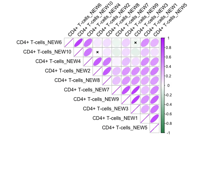
# 查看模块相关图
ModuleCorrelogram(seurat_obj)

不同hMEs模块在不同细胞细胞群中的情况，笔者这里仅作演示。真实分析的时候不能这样展示，因为笔者仅用了CD4+ T细胞作的hdWGCNA，因此不应该映射到全部的细胞亚群。

hub scores展示，跟上面异曲同工了。

雷达图，这里说明了不同模块在不同样本中的百分比情况，这里可以改成更精细的细胞亚群。

不同模块之间的相关性分析。

6.其他可视化

气泡图

# get hMEs from seurat object
MEs <- GetMEs(seurat_obj, harmonized=TRUE)
modules <- GetModules(seurat_obj)
mods <- levels(modules$module); mods <- mods[mods != 'grey']

# add hMEs to Seurat meta-data:
seurat_obj@meta.data <- cbind(seurat_obj@meta.data, MEs)

# plot with Seurat's DotPlot function
p <- DotPlot(seurat_obj, features=mods, group.by = 'celltype')

# flip the x/y axes, rotate the axis labels, and change color scheme:
p <- p +
  RotatedAxis() +
  scale_color_gradient2(high='red', mid='grey95', low='blue')

# plot output
p

不同hMEs模块在不同细胞细胞群中的气泡图，同样仅做展示，真实分析的时候不能这么做。

模块的网络图

# 使用ModuleNetworkPlot可视化每个模块前50(数值可自定)的hub gene
ModuleNetworkPlot(
    seurat_obj, 
    outdir='ModuleNetworks', # new folder name
    n_inner = 20, # number of genes in inner ring
    n_outer = 30, # number of genes in outer ring
    n_conns = Inf, # show all of the connections
    plot_size=c(10,10), # larger plotting area
    vertex.label.cex=1 # font size
)

结合hub基因的网络图

# hubgene network(基因数可自定)
HubGeneNetworkPlot(
  seurat_obj,
  n_hubs = 2, 
  n_other=2,
  edge_prop = 0.75,
  mods = 'all'
)
# 超内存了，笔记本扛不住
# Error in getGlobalsAndPackages(expr, envir = envir, globals = globals) : 
#   The total size of the 4 globals exported for future expression (‘FUN()’) is 1.52 GiB.. This exceeds the maximum allowed size of 500.00 MiB (option 'future.globals.maxSize'). The three largest globals are ‘FUN’ (1.52 GiB of class ‘function’), ‘modules’ (1.07 MiB of class ‘list’) and ‘edge_df’ (11.39 KiB of class ‘list’)


# 可以选择模块数
g <- HubGeneNetworkPlot(seurat_obj,  return_graph=TRUE)
# get the list of modules:
modules <- GetModules(seurat_obj)
mods <- levels(modules$module); mods <- mods[mods != 'grey']
# hubgene network
HubGeneNetworkPlot(
  seurat_obj,
  n_hubs = 2, 
  n_other= 2,
  edge_prop = 0.75,
  mods = mods[1:5] # only select 5 modules
)

笔者的笔记本运行内存比较小，这里的图片画不出来了，以下是官网示例图。

UMAP-共表达网络图

seurat_obj <- RunModuleUMAP(
  seurat_obj,
  n_hubs = 10, # number of hub genes to include for the UMAP embedding
  n_neighbors=15, # neighbors parameter for UMAP
  min_dist=0.1 # min distance between points in UMAP space
)

# get the hub gene UMAP table from the seurat object
umap_df <- GetModuleUMAP(seurat_obj)

# plot with ggplot
ggplot(umap_df, aes(x=UMAP1, y=UMAP2)) +
  geom_point(
   color=umap_df$color, # color each point by WGCNA module
   size=umap_df$kME*2 # size of each point based on intramodular connectivity
  ) +
  umap_theme()


ModuleUMAPPlot(
  seurat_obj,
  edge.alpha=0.25,
  sample_edges=TRUE,
  edge_prop=0.1, # proportion of edges to sample (20% here)
  label_hubs=2 ,# how many hub genes to plot per module?
  keep_grey_edges=FALSE
)
# [1] "hub labels"
#  [1] "RPS13"   "RPS15A"  "GIMAP4"  "SLFN5"   "FBN1"    "RAB31"   "SMAP2"  
#  [8] "CNOT6L"  "CHCHD2"  "PSMA7"   "CREM"    "SRGN"    "KLHDC3"  "TMEM147"
# [15] "MLLT10"  "CHD3"    "HSPA1A"  "MT2A"    "DNAJA1"  "JUND"   
# NULL
#  [1] "RPS13"   "RPS15A"  "GIMAP4"  "SLFN5"   "FBN1"    "RAB31"   "SMAP2"  
#  [8] "CNOT6L"  "CHCHD2"  "PSMA7"   "CREM"    "SRGN"    "KLHDC3"  "TMEM147"
# [15] "MLLT10"  "CHD3"    "HSPA1A"  "MT2A"    "DNAJA1"  "JUND"   
# [1] 362100      3
# Error in getGlobalsAndPackages(expr, envir = envir, globals = globals) : 
#   The total size of the 3 globals exported for future expression (‘FUN()’) is 1.54 GiB.. This exceeds the maximum allowed size of 500.00 MiB (option 'future.globals.maxSize'). There are three globals: ‘FUN’ (1.53 GiB of class ‘function’), ‘edge_df’ (5.57 MiB of class ‘list’) and ‘selected_modules’ (727.23 KiB of class ‘list’)

笔者的笔记本运行内存比较小，这里的图片画不出来了，以下是官网示例图。

7.可选可视化

可视化方案特别多，可点击参考资料查看~

g <- ModuleUMAPPlot(seurat_obj,  return_graph=TRUE)

# run supervised UMAP:
seurat_obj <- RunModuleUMAP(
  seurat_obj,
  n_hubs = 10,
  n_neighbors=15,
  min_dist=0.1,
  supervised=TRUE,
  target_weight=0.5
)

# get the hub gene UMAP table from the seurat object
umap_df <- GetModuleUMAP(seurat_obj)

# plot with ggplot
ggplot(umap_df, aes(x=UMAP1, y=UMAP2)) +
  geom_point(
   color=umap_df$color, # color each point by WGCNA module
   size=umap_df$kME*2 # size of each point based on intramodular connectivity
  ) +
  umap_theme()

自定义网络图

请自行修改内部参数

# load the packages:
library(ggraph)
library(tidygraph)

# get modules and TOM from the seurat obj
modules <- GetModules(seurat_obj) %>% 
  subset(module != 'grey') %>% 
  mutate(module = droplevels(module))
mods <- levels(modules$module)
TOM <- GetTOM(seurat_obj)

# get module colors for plotting 
mod_colors <- dplyr::select(modules, c(module, color)) %>% distinct()
mod_cp <- mod_colors$color; names(mod_cp) <- as.character(mod_colors$module)

# load the GO Biological Pathways file (donwloaded from EnrichR website)
pathways <- fgsea::gmtPathways('GO_Biological_Process_2021.txt')

# remove GO Term ID for simplicity:
names(pathways) <- stringr::str_replace(names(pathways), " \\s*\\([^\\)]+\\)", "")

# selected pathway 
cur_pathway <- 'nervous system development'

# get genes in this pathway 
cur_genes <- pathways[[cur_pathway]]
cur_genes <- cur_genes[cur_genes %in% modules$gene_name]

# subset the TOM 
cur_TOM <- TOM[cur_genes,cur_genes] 

# 使用ggraph绘制基本网络图
# set up the graph object with igraph & tidygraph
graph <- cur_TOM %>% 
  igraph::graph_from_adjacency_matrix(mode='undirected', weighted=TRUE) %>% 
  tidygraph::as_tbl_graph(directed=FALSE) %>% 
  tidygraph::activate(nodes) 

# make the plot with ggraph
p <- ggraph(graph) + 
  geom_edge_link(color='grey', alpha=0.2) + 
  geom_node_point(color='black') +
  geom_node_label(aes(label=name), repel=TRUE, max.overlaps=Inf, fontface='italic') 
p

# ggraph第2种方式
# set up the graph object with igraph & tidygraph
graph <- cur_TOM %>% 
  igraph::graph_from_adjacency_matrix(mode='undirected', weighted=TRUE) %>% 
  tidygraph::as_tbl_graph(directed=FALSE) %>% 
  tidygraph::activate(nodes) 

# add the module name to the graph:
V(graph)$module <- modules[V(graph)$name,'module']

# make the plot with gggraph
p <- ggraph(graph) + 
  geom_edge_link(aes(alpha=weight), color='grey') + 
  geom_node_point(aes(color=module)) +
  geom_node_label(aes(label=name), repel=TRUE, max.overlaps=Inf, fontface='italic') +
  scale_colour_manual(values=mod_cp)  
p

Manipulating the network

# only keep the upper triangular part of the TOM:
cur_TOM[upper.tri(cur_TOM)] <- NA

# cast the network from wide to long format
cur_network <- cur_TOM %>% 
  reshape2::melt() %>% 
  dplyr::rename(gene1 = Var1, gene2 = Var2, weight=value) %>%
  subset(!is.na(weight))

# get the module & color info for gene1
temp1 <- dplyr::inner_join(
  cur_network,
  modules %>% 
    dplyr::select(c(gene_name, module, color)) %>% 
    dplyr::rename(gene1 = gene_name, module1=module, color1=color),
  by = 'gene1'
) %>% dplyr::select(c(module1, color1))

# get the module & color info for gene2
temp2 <- dplyr::inner_join(
  cur_network,
  modules %>% 
    dplyr::select(c(gene_name, module, color)) %>% 
    dplyr::rename(gene2 = gene_name, module2=module, color2=color),
  by = 'gene2'
) %>% dplyr::select(c(module2, color2))

# add the module & color info 
cur_network <- cbind(cur_network, temp1, temp2)

# set the edge color to the module's color if they are the two genes are in the same module 
cur_network$edge_color <- ifelse(
  cur_network$module1 == cur_network$module2, 
  as.character(cur_network$module1),
  'grey'
)

# keep this network before subsetting
cur_network_full <- cur_network 

# keep the top 10% of edges 
edge_percent <- 0.1
cur_network <- cur_network_full %>% 
  dplyr::slice_max(
    order_by = weight, 
    n = round(nrow(cur_network)*edge_percent)
  )

# make the graph object with tidygraph
graph <- cur_network %>% 
  igraph::graph_from_data_frame() %>%
  tidygraph::as_tbl_graph(directed=FALSE) %>% 
  tidygraph::activate(nodes)

# add the module name to the graph:
V(graph)$module <- modules[V(graph)$name,'module']

# get the top 25 hub genes for each module
hub_genes <- GetHubGenes(seurat_obj, n_hubs=25) %>% .$gene_name
V(graph)$hub <- ifelse(V(graph)$name %in% hub_genes, V(graph)$name, "")

# make the plot with gggraph
p <- ggraph(graph) + 
  geom_edge_link(aes(alpha=weight, color=edge_color)) + 
  geom_node_point(aes(color=module)) +
  geom_node_label(aes(label=hub), repel=TRUE, max.overlaps=Inf, fontface='italic') +
  scale_colour_manual(values=mod_cp) +
  scale_edge_colour_manual(values=mod_cp) 

p


# 第二种方式
# subset to only keep edges between genes in the same module
cur_network <- cur_network_full %>% 
  subset(module1 == module2)

# make the graph object with tidygraph
graph <- cur_network %>% 
  igraph::graph_from_data_frame() %>%
  tidygraph::as_tbl_graph(directed=FALSE) %>% 
  tidygraph::activate(nodes)

# add the module name to the graph:
V(graph)$module <- modules[V(graph)$name,'module']

# get the top 25 hub genes for each module
hub_genes <- GetHubGenes(seurat_obj, n_hubs=25) %>% .$gene_name
V(graph)$hub <- ifelse(V(graph)$name %in% hub_genes, V(graph)$name, "")

# make the plot with gggraph
p <- ggraph(graph) + 
  geom_edge_link(aes(alpha=weight, color=edge_color)) + 
  geom_node_point(aes(color=module)) +
  geom_node_label(aes(label=hub), repel=TRUE, max.overlaps=Inf, fontface='italic') +
  scale_colour_manual(values=mod_cp) +
  scale_edge_colour_manual(values=mod_cp) +
  NoLegend()

p

Specifying network layouts

# randomly sample 50% of the edges within the same module
cur_network1 <- cur_network_full %>% 
  subset(module1 == module2) %>%
  group_by(module1) %>%
  sample_frac(0.5) %>% 
  ungroup()

# keep the top 10% of other edges 
edge_percent <- 0.10
cur_network2 <- cur_network_full %>% 
  subset(module1 != module2) %>%
  dplyr::slice_max(
    order_by = weight, 
    n = round(nrow(cur_network)*edge_percent)
  )

cur_network <- rbind(cur_network1, cur_network2)

# set factor levels for edges:
cur_network$edge_color <- factor(
  as.character(cur_network$edge_color),
  levels = c(mods, 'grey')
)

# rearrange so grey edges are on the bottom:
cur_network %<>% arrange(rev(edge_color))

# make the graph object with tidygraph
graph <- cur_network %>% 
  igraph::graph_from_data_frame() %>%
  tidygraph::as_tbl_graph(directed=FALSE) %>% 
  tidygraph::activate(nodes)

# add the module name to the graph:
V(graph)$module <- modules[V(graph)$name,'module']

# get the top 25 hub genes for each module
hub_genes <- GetHubGenes(seurat_obj, n_hubs=25) %>% .$gene_name
V(graph)$hub <- ifelse(V(graph)$name %in% hub_genes, V(graph)$name, "")

# 1. default layout
p1 <- ggraph(graph) + 
  geom_edge_link(aes(alpha=weight, color=edge_color)) + 
  geom_node_point(aes(color=module)) +
  scale_colour_manual(values=mod_cp) +
  scale_edge_colour_manual(values=mod_cp) +
  ggtitle("layout = 'stress' (auto)") +
  NoLegend()

# 2. Kamada Kawai (kk) layout
graph2 <- graph; E(graph)$weight <- E(graph)$weight + 0.0001
p2 <- ggraph(graph, layout='kk', maxiter=100) + 
  geom_edge_link(aes(alpha=weight, color=edge_color)) + 
  geom_node_point(aes(color=module)) +
  scale_colour_manual(values=mod_cp) +
  scale_edge_colour_manual(values=mod_cp) +
  ggtitle("layout = 'kk'") +
  NoLegend()

# 3. igraph layout_with_fr
p3 <- ggraph(graph, layout=layout_with_fr(graph)) + 
  geom_edge_link(aes(alpha=weight, color=edge_color)) + 
  geom_node_point(aes(color=module)) +
  scale_colour_manual(values=mod_cp) +
  scale_edge_colour_manual(values=mod_cp) +
  ggtitle("layout_with_fr()") +
  NoLegend()

# 4. igraph layout_as_tree
p4 <- ggraph(graph, layout=layout_as_tree(graph)) + 
  geom_edge_link(aes(alpha=weight, color=edge_color)) + 
  geom_node_point(aes(color=module)) +
  scale_colour_manual(values=mod_cp) +
  scale_edge_colour_manual(values=mod_cp) +
  ggtitle("layout_as_tree()") +
  NoLegend()

# 5. igraph layout_nicely
p5 <- ggraph(graph, layout=layout_nicely(graph)) + 
  geom_edge_link(aes(alpha=weight, color=edge_color)) + 
  geom_node_point(aes(color=module)) +
  scale_colour_manual(values=mod_cp) +
  scale_edge_colour_manual(values=mod_cp) +
  ggtitle("layout_nicely()") +
  NoLegend()

# 6. igraph layout_in_circle
p6 <- ggraph(graph, layout=layout_in_circle(graph)) + 
  geom_edge_link(aes(alpha=weight, color=edge_color)) + 
  geom_node_point(aes(color=module)) +
  scale_colour_manual(values=mod_cp) +
  scale_edge_colour_manual(values=mod_cp) +
  ggtitle("layout_in_circle()") +
  NoLegend()


# make a combined plot
(p1 | p2 | p3) / (p4 | p5 | p6) 

##########################
# get the UMAP df and subset by genes that are in our graph
umap_df <- GetModuleUMAP(seurat_obj)
umap_layout <- umap_df[names(V(graph)),] %>% dplyr::rename(c(x=UMAP1, y = UMAP2, name=gene))
rownames(umap_layout) <- 1:nrow(umap_layout)

# create the layout
lay <- ggraph::create_layout(graph, umap_layout)
lay$hub <- V(graph)$hub

p <- ggraph(lay) + 
  geom_edge_link(aes(alpha=weight, color=edge_color)) +
  geom_node_point(data=subset(lay, hub == ''), aes(color=module, size=kME)) + 
  geom_node_point(data=subset(lay, hub != ''), aes(fill=module, size=kME), color='black', shape=21) +
  scale_colour_manual(values=mod_cp) +
  scale_fill_manual(values=mod_cp) +
  scale_edge_colour_manual(values=mod_cp) +
  geom_node_label(aes(label=hub), repel=TRUE, max.overlaps=Inf, fontface='italic') +
  NoLegend()
p 

######################
p <- ggraph(lay) + 
  ggrastr::rasterise(
    geom_point(inherit.aes=FALSE, data=umap_df, aes(x=UMAP1, y=UMAP2), color=umap_df$color, alpha=0.1, size=1),
    dpi=500
   ) +
  geom_edge_link(aes(alpha=weight, color=edge_color)) +
  geom_node_point(data=subset(lay, hub == ''), aes(fill=module, size=kME), color='black', shape=21) + 
  geom_node_point(data=subset(lay, hub != ''), aes(fill=module, size=kME), color='black', shape=23) +
  scale_colour_manual(values=mod_cp) +
  scale_fill_manual(values=mod_cp) +
  scale_edge_colour_manual(values=mod_cp) +
  geom_node_label(aes(label=hub), repel=TRUE, max.overlaps=Inf, fontface='italic') +
  NoLegend()

####################
p <- ggraph(lay) + 
  ggrastr::rasterise(
    geom_point(inherit.aes=FALSE, data=umap_df, aes(x=UMAP1, y=UMAP2), color=umap_df$color, alpha=0.1, size=1),
    dpi=500
   ) +
  geom_edge_link(aes(alpha=weight, color=edge_color)) +
  geom_node_point(data=subset(lay, hub == ''), aes(fill=module, size=kME), color='black', shape=21) + 
  geom_node_point(data=subset(lay, hub != ''), aes(fill=module, size=kME), color='black', shape=23) +
  scale_colour_manual(values=mod_cp) +
  scale_fill_manual(values=mod_cp) +
  scale_edge_colour_manual(values=mod_cp) +
  geom_node_label(aes(label=hub, color=module), repel=TRUE, max.overlaps=Inf, fontface='italic') +
  NoLegend()

p <- p + 
  theme(
    panel.background = element_rect(fill='black'),
    plot.title = element_text(hjust=0.5)
  ) + 
  annotate("text", x=Inf, y=Inf, label="Nervous system development", 
  vjust=2, hjust=1.1, color='white', fontface='bold', size=5)

p

总之花里胡哨的可视化很多，但是真正我们需要的仅仅是关键模块和内部的基因~