


scMetabolism一个单细胞水平的代谢相关通路分析工具。
内置了KEGG_metabolism_nc和REACTOME_metabolism两个库的代谢通路信息。
分析方法可选择VISION、AUCell、ssgsea和gsva这四种,默认是VISION。
其他没有什么需要特殊介绍的。
分析流程
1.导入
rm(list = ls())
# V5_path = "/Library/Frameworks/R.framework/Versions/4.4-arm64/Resources/seurat5/"
# .libPaths(V5_path)
# .libPaths()
library(stringr)
library(Seurat)
library(rsvd)
library(qs)
library(scMetabolism)
library(BiocParallel)
register(MulticoreParam(workers = 4, progressbar = TRUE))

scRNA <- qread("sc_dataset.qs") # V4 data
sub_scRNA <- subset(scRNA,
                    subset = celltype %in% c("epithelial/cancer cells",
                                              "myeloid cells"))
load("scRNA.Rdata") # V5 data
2.V5版本(需修改代码)
sc.metabolism.SeuratV5 <- function (obj, method = "VISION", imputation = F, ncores = 2,
  metabolism.type = "KEGG")
{
  countexp <- GetAssayData(obj, layer='counts')
  countexp <- data.frame(as.matrix(countexp))
  signatures_KEGG_metab <- system.file("data", "KEGG_metabolism_nc.gmt",
    package = "scMetabolism")
  signatures_REACTOME_metab <- system.file("data", "REACTOME_metabolism.gmt",
    package = "scMetabolism")
  if (metabolism.type == "KEGG") {
    gmtFile <- signatures_KEGG_metab
    cat("Your choice is: KEGG\n")
  }
  if (metabolism.type == "REACTOME") {
    gmtFile <- signatures_REACTOME_metab
    cat("Your choice is: REACTOME\n")
  }
  if (imputation == F) {
    countexp2 <- countexp
  }
  if (imputation == T) {
    cat("Start imputation...\n")
    cat("Citation: George C. Linderman, Jun Zhao, Yuval Kluger. Zero-preserving imputation of scRNA-seq data using low-rank approximation. bioRxiv. doi: https://doi.org/10.1101/397588 \n")
    result.completed <- alra(as.matrix(countexp))
    countexp2 <- result.completed[[3]]
    row.names(countexp2) <- row.names(countexp)
  }
  cat("Start quantify the metabolism activity...\n")
  if (method == "VISION") {
    library(VISION)
    n.umi <- colSums(countexp2)
    scaled_counts <- t(t(countexp2)/n.umi) * median(n.umi)
    vis <- Vision(scaled_counts, signatures = gmtFile)
    options(mc.cores = ncores)
    vis <- analyze(vis)
    signature_exp <- data.frame(t(vis@SigScores))
  }
  if (method == "AUCell") {
    library(AUCell)
    library(GSEABase)
    cells_rankings <- AUCell_buildRankings(as.matrix(countexp2),
      nCores = ncores, plotStats = F)
    geneSets <- getGmt(gmtFile)
    cells_AUC <- AUCell_calcAUC(geneSets, cells_rankings)
    signature_exp <- data.frame(getAUC(cells_AUC))
  }
  if (method == "ssGSEA") {
    library(GSVA)
    library(GSEABase)
    geneSets <- getGmt(gmtFile)
    gsva_es <- gsva(as.matrix(countexp2), geneSets, method = c("ssgsea"),
      kcdf = c("Poisson"), parallel.sz = ncores)
    signature_exp <- data.frame(gsva_es)
  }
  if (method == "ssGSEA") {
    library(GSVA)
    library(GSEABase)
    geneSets <- getGmt(gmtFile)
    gsva_es <- gsva(as.matrix(countexp2), geneSets, method = c("gsva"),
      kcdf = c("Poisson"), parallel.sz = ncores)
    signature_exp <- data.frame(gsva_es)
  }
  cat("\nPlease Cite: \nYingcheng Wu, Qiang Gao, et al. Cancer Discovery. 2021. \nhttps://pubmed.ncbi.nlm.nih.gov/34417225/   \n\n")
  obj@assays$METABOLISM$score <- signature_exp
  obj
}

Idents(scRNA) <- "celltype"
res <-sc.metabolism.SeuratV5(obj = scRNA,
                             method = "VISION", # VISION、AUCell、ssgsea和gsva
                             imputation =F, ncores = 2,
                             metabolism.type = "KEGG") # KEGG和REACTOME
3.V5可视化(需修改代码)
# 需要修改DimPlot.metabolism中的UMAP大小写
DimPlot.metabolismV5 <- function (obj, pathway, dimention.reduction.type = "umap", dimention.reduction.run = T,
size = 1)
{
cat("\nPlease Cite: \nYingcheng Wu, Qiang Gao, et al. Cancer Discovery. 2021. \nhttps://pubmed.ncbi.nlm.nih.gov/34417225/ \n\n")
if (dimention.reduction.type == "umap") {
if (dimention.reduction.run == T)
obj <- Seurat::RunUMAP(obj, reduction = "pca", dims = 1:40)
umap.loc <- obj@reductions$umap@cell.embeddings
row.names(umap.loc) <- colnames(obj)
signature_exp <- obj@assays$METABOLISM$score
input.pathway <- pathway
signature_ggplot <- data.frame(umap.loc, t(signature_exp[input.pathway,
]))
library(wesanderson)
pal <- wes_palette("Zissou1", 100, type = "continuous")
library(ggplot2)
plot <- ggplot(data = signature_ggplot, aes(x = umap_1,
y = umap_2, color = signature_ggplot[, 3])) + geom_point(size = size) +
scale_fill_gradientn(colours = pal) + scale_color_gradientn(colours = pal) +
labs(color = input.pathway) + xlab("UMAP 1") + ylab("UMAP 2") +
theme(aspect.ratio = 1) + theme(panel.grid.major = element_blank(),
panel.grid.minor = element_blank(), panel.background = element_blank(),
axis.line = element_line(colour = "black"))
}
if (dimention.reduction.type == "tsne") {
if (dimention.reduction.run == T)
obj <- Seurat::RunTSNE(obj, reduction = "pca", dims = 1:40)
tsne.loc <- obj@reductions$tsne@cell.embeddings
row.names(tsne.loc) <- colnames(obj)
signature_exp <- obj@assays$METABOLISM$score
input.pathway <- pathway
signature_ggplot <- data.frame(tsne.loc, t(signature_exp[input.pathway,
]))
pal <- wes_palette("Zissou1", 100, type = "continuous")
library(ggplot2)
plot <- ggplot(data = signature_ggplot, aes(x = tSNE_1,
y = tSNE_2, color = signature_ggplot[, 3])) + geom_point(size = size) +
scale_fill_gradientn(colours = pal) + scale_color_gradientn(colours = pal) +
labs(color = input.pathway) + xlab("tSNE 1") + ylab("tSNE 2") +
theme(aspect.ratio = 1) + theme(panel.grid.major = element_blank(),
panel.grid.minor = element_blank(), panel.background = element_blank(),
axis.line = element_line(colour = "black"))
}
plot
}
# check一下有哪些pathway
pathways <- res@assays$METABOLISM$score
head(rownames(pathways))
# [1] "Glycolysis / Gluconeogenesis"
# [2] "Citrate cycle (TCA cycle)"
# [3] "Pentose phosphate pathway"
# [4] "Pentose and glucuronate interconversions"
# [5] "Fructose and mannose metabolism"
# [6] "Galactose metabolism"
# Dimplot
DimPlot.metabolismV5(obj = res,
pathway = "Glycolysis / Gluconeogenesis",
dimention.reduction.type = "umap",
dimention.reduction.run = F, size = 1)
# DotPlot
input.pathway<-c("Glycolysis / Gluconeogenesis",
"Oxidative phosphorylation",
"Citrate cycle (TCA cycle)")
DotPlot.metabolism(obj = res,
pathway = input.pathway,
phenotype = "celltype", #这个参数需按需修改
norm = "y")
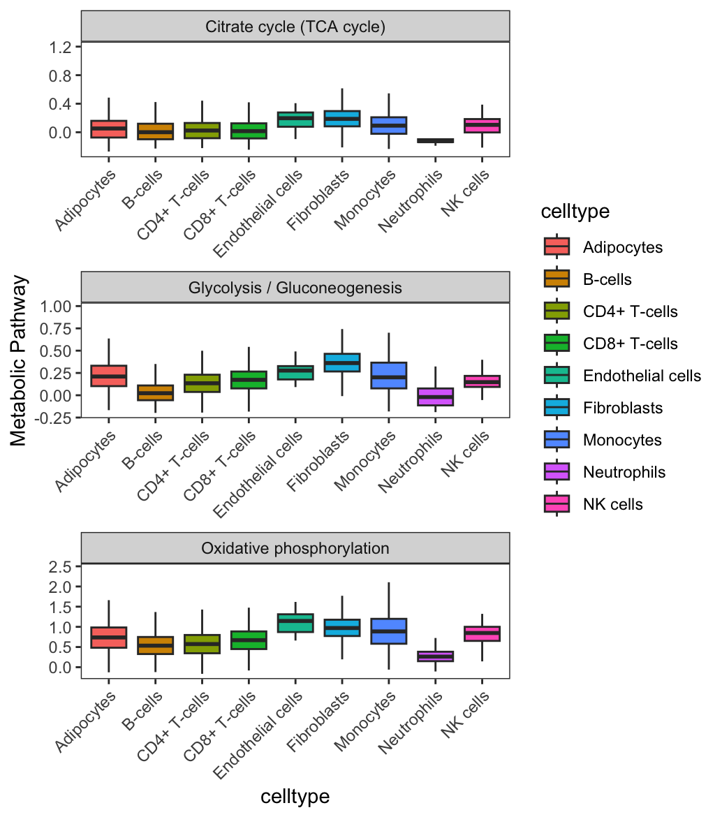
# BoxPlot
# 由于开发者默认吧obj定义为countexp.Seurat,所以还需要重新命名一下
countexp.Seurat <- res
BoxPlot.metabolism(obj = countexp.Seurat,
pathway = input.pathway,
phenotype = "celltype", #这个参数需按需修改
ncol = 1)


4.V4可直接用
res <-sc.metabolism.Seurat(obj = sub_scRNA,
                           method = "AUCell", # VISION、AUCell、ssgsea和gsva
                           imputation =F, ncores = 2,
                           metabolism.type = "KEGG") # KEGG和REACTOME
5.V4可视化
# check一下有哪些pathway
pathways <- res@assays$METABOLISM$score
head(rownames(pathways))
# [1] "Terpenoid backbone biosynthesis"
# [2] "Caffeine metabolism"
# [3] "Neomycin, kanamycin and gentamicin biosynthesis"
# [4] "Metabolism of xenobiotics by cytochrome P450"
# [5] "Drug metabolism - cytochrome P450"
# [6] "Drug metabolism - other enzymes"

# Dimplot绘图
DimPlot.metabolism(obj = res,
                   pathway = "Glycolysis / Gluconeogenesis",
                   dimention.reduction.type = "umap",
                   dimention.reduction.run = F, size = 1)

# DotPlot
input.pathway<-c("Folate biosynthesis",
                 "Nicotinate and nicotinamide metabolism",
                 "Pyrimidine metabolism")
DotPlot.metabolism(obj = res,
                  pathway = input.pathway,
                  phenotype = "celltype", #这个参数需按需修改
                  norm = "y")

#BoxPlot
# 由于开发者默认吧obj定义为countexp.Seurat,所以还需要重新命名一下
countexp.Seurat <- res
BoxPlot.metabolism(obj = countexp.Seurat,
                  pathway = input.pathway,
                  phenotype = "celltype", #这个参数需按需修改
                  ncol = 1)


参考资料:
1、Spatiotemporal Immune Landscape of Colorectal Cancer Liver Metastasis at Single-Cell Level. Cancer Discov. 2022 Jan;12(1):134-153.
2、scMetabolism: https://github.com/wu-yc/scMetabolism
3、生信菜鸟团:
https://mp.weixin.qq.com/s/nSXm3gDBu9be2vogFnYxbQ;
https://mp.weixin.qq.com/s/CG4cWARe9KegD-gqz0rDzw
注:若对内容有疑惑或者有发现明确错误的朋友,请联系后台(欢迎交流)。更多内容可关注公众号:生信方舟
- END -


 2444
2444

 被折叠的 条评论
为什么被折叠?
被折叠的 条评论
为什么被折叠?
 到【灌水乐园】发言


