


1、本模型所用函数包
2、数据集
3、模型框架
4、测试自己的图片
第一门课:神经网络和深度学习
第四周:深层神经网络
一、函数包
import time
import numpy as np
import h5py  # h5py是一个与h5文件交互常用的函数包
import matplotlib.pyplot as plt  # PIL用于在最后使用自己的图片测试自己的模型
import scipy
from PIL import Image
from scipy import ndimage
from dnn_app_utils_v2 import *  # dnn_app_utils提供了构建神经网络所需要的函数:在上个编程任务中实现的函数

plt.rcParams['figure.figsize'] = (5.0, 4.0)  # set default size of plots
plt.rcParams['image.interpolation'] = 'nearest'
plt.rcParams['image.cmap'] = 'gray'
np.random.seed(1)
二、数据集
问题表述:
数据集(“data.h5”),其中包括:m_train个具有猫\非猫标注的图片训练集,m_test个具有猫\非猫标注的图片测试集
每张图片的维度都是(num_px,num_px,3),其中3是3个RGB通道
# 加载数据集
train_x_orig, train_y, test_x_orig, test_y, classes = load_data()
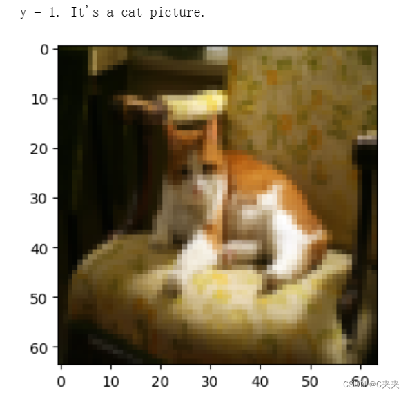
# 示例图片
index = 7
plt.imshow(train_x_orig[index])
print("y = " + str(train_y[0, index]) + ". It's a " + classes[train_y[0, index]].decode("utf-8") + " picture.")
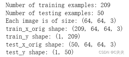
# 探索数据集
m_train = train_x_orig.shape[0]
num_px = train_x_orig.shape[1]
m_test = test_x_orig.shape[0]
print("训练集数量: " + str(m_train))
print("测试集数量: " + str(m_test))
print("每张图片的尺寸: (" + str(num_px) + ", " + str(num_px) + ", 3)")
print("train_x_orig 尺寸: " + str(train_x_orig.shape))
print("train_y 尺寸: " + str(train_y.shape))
print("test_x_orig 尺寸: " + str(test_x_orig.shape))
print("test_y 尺寸: " + str(test_y.shape))
# reshape照片的维度并且使其标准化再将他们放到网络中去训练
# 重塑训练集与测试集维度
train_x_flatten = train_x_orig.reshape(train_x_orig.shape[0], -1).T  # "-1" 让reshape展平剩余尺寸
test_x_flatten = test_x_orig.reshape(test_x_orig.shape[0], -1).T
# 标准化数据让特征值在0-1之间
train_x = train_x_flatten / 255.
test_x = test_x_flatten / 255.
print("train_x's 尺寸: " + str(train_x.shape))
print("test_x's 尺寸: " + str(test_x.shape))  # 12288 = 64*64*3
12,288= 64×64×3,which is the size of one reshaped image vector.
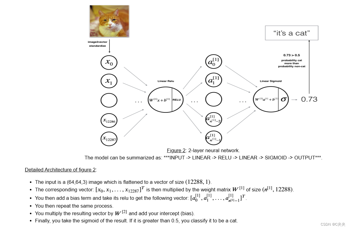
三、模型框架
构建两个不同模型-2层神经网络模型、L层神经网络模型
构建网络的常规方法:
1)初始化参数/定义超参数
2)循环遍历num_iterations:前向传播—计算损失函数—后向传播—更新参数(使用参数和从backprop中的grads)
3)使用训练参数来预测标签
1、两层神经网络
使用之前实现的辅助函数构建两层神经网络LINEAR -> RELU -> LINEAR -> SIGMOID
# 模型的参数设定
n_x = 12288 # num_px * num_px * 3
n_h = 7
n_y = 1
layers_dims = (n_x, n_h, n_y)
# 两层神经网络的实现
"""
Arguments:
X -- 输入数据, 尺寸 (n_x, 示例数)
Y -- 真值标签向量 (是猫为0,不是猫为1), 尺寸 (1, 示例数)
层数 -- 层尺寸 (n_x, n_h, n_y)
num_iterations -- 优化循环的迭代次数
learning_rate -- 梯度下降更新规则的学习率
print_cost -- 如果设置为真,将每100迭代绘制出代价
Returns:
parameters -- 一个包含 W1, W2, b1, and b2的字典
"""
def two_layer_model(X, Y, layers_dims, learning_rate=0.0075, num_iterations=3000, print_cost=False):
np.random.seed(1)
grads = {}
costs = [] # 跟踪代价
m = X.shape[1] # 示例数
(n_x, n_h, n_y) = layers_dims
# 通过之前实现的函数初始化参数
parameters = initialize_parameters(n_x, n_h, n_y)
# 从字典中得到W1, b1, W2 and b2
W1 = parameters["W1"]
b1 = parameters["b1"]
W2 = parameters["W2"]
b2 = parameters["b2"]
# 梯度下降
for i in range(0, num_iterations):
# 前向传播:LINEAR -> RELU -> LINEAR -> SIGMOID
# Inputs: "X, W1, b1". Output: "A1, cache1, A2, cache2
A1, cache1 = linear_activation_forward(X, W1, b1, activation="relu")
A2, cache2 = linear_activation_forward(A1, W2, b2, activation="sigmoid")
# 计算代价
cost = compute_cost(A2, Y)
# 初始化后向传播
dA2 = - (np.divide(Y, A2) - np.divide(1 - Y, 1 - A2))
# 后向传播,Inputs: "dA2, cache2, cache1". Outputs: "dA1, dW2, db2; also dA0, dW1, db1"
dA1, dW2, db2 = linear_activation_backward(dA2, cache2, activation="sigmoid")
dA0, dW1, db1 = linear_activation_backward(dA1, cache1, activation="relu")
# Set grads['dWl'] to dW1, grads['db1'] to db1, grads['dW2'] to dW2, grads['db2'] to db2
grads['dW1'] = dW1
grads['db1'] = db1
grads['dW2'] = dW2
grads['db2'] = db2
# 更新参数
W1, b1, W2, b2 = update_parameters(parameters, grads, learning_rate)
# Retrieve W1, b1, W2, b2 from parameters
W1 = parameters["W1"]
b1 = parameters["b1"]
W2 = parameters["W2"]
b2 = parameters["b2"]
# Print the cost every 100 training example
if print_cost and i % 100 == 0:
print("Cost after iteration {}: {}".format(i, np.squeeze(cost)))
if print_cost and i % 100 == 0:
costs.append(cost)
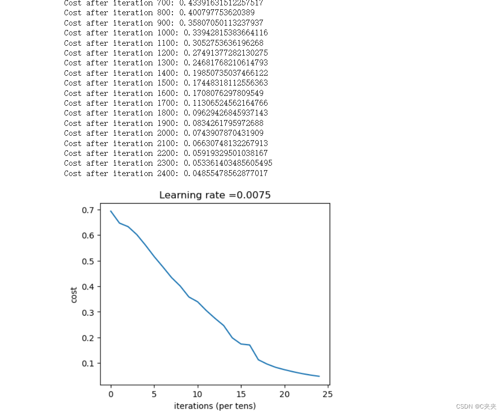
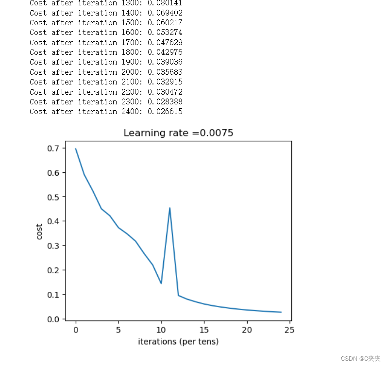
# plot the cost
plt.plot(np.squeeze(costs))
plt.ylabel('cost')
plt.xlabel('iterations (per tens)')
plt.title("学习率 =" + str(learning_rate))
plt.show()
return parameters
parameters = two_layer_model(train_x, train_y, layers_dims = (n_x, n_h, n_y), num_iterations = 2500, print_cost=True)
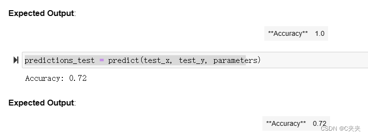
predictions_train = predict(train_x, train_y, parameters)
predictions_test = predict(test_x, test_y, parameters)
输出结果为:
2、L层神经网络
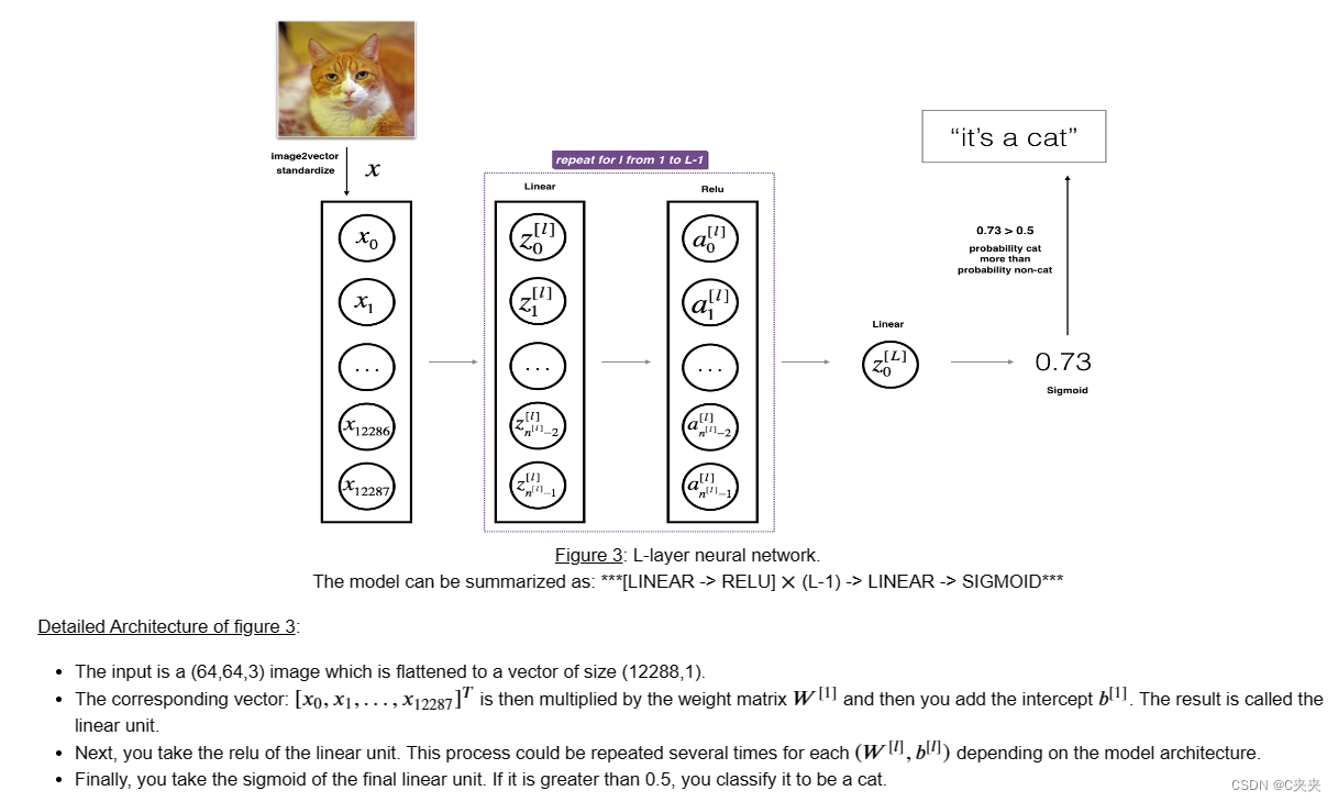
# 使用之前实现的辅助函数[LINEAR -> RELU]$\times$(L-1) -> LINEAR -> SIGMOID
layers_dims = [12288, 20, 7, 5, 1]    # 5层模型
def L_layer_model(X, Y, layers_dims, learning_rate=0.0075, num_iterations=3000, print_cost=False):  # lr was 0.009
    np.random.seed(1)
    costs = []
    # Parameters initialization.
    parameters = initialize_parameters_deep(layers_dims)
    # Loop (gradient descent)
    for i in range(0, num_iterations):
        # Forward propagation: [LINEAR -> RELU]*(L-1) -> LINEAR -> SIGMOID.
        AL, caches = L_model_forward(X, parameters)#
        # Compute cost.
        cost = compute_cost(AL, Y)
        # Backward propagation.
        grads = L_model_backward(AL, Y, caches)
        # Update parameters.
        parameters = update_parameters(parameters, grads, learning_rate)
        # Print the cost every 100 training example
        if print_cost and i % 100 == 0:
            print("Cost after iteration %i: %f" % (i, cost))
        if print_cost and i % 100 == 0:
            costs.append(cost)
    # plot the cost
    plt.plot(np.squeeze(costs))
    plt.ylabel('cost')
    plt.xlabel('iterations (per tens)')
    plt.title("Learning rate =" + str(learning_rate))
    plt.show()
    return parameters
parameters = L_layer_model(train_x, train_y, layers_dims, num_iterations = 2500, print_cost = True)
pred_train = predict(train_x, train_y, parameters)
pred_test = predict(test_x, test_y, parameters)
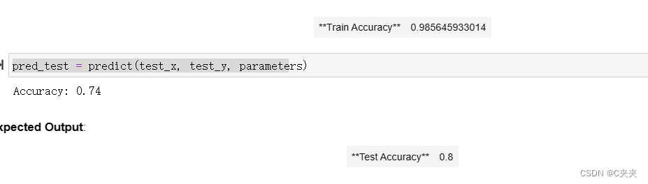
结果分析
一些在模型中被错误分类图片的特征:
1、猫的身体处于异常的位置
2、猫出现在与自身颜色相似的背景中
3、猫有不寻常的颜色和品种
4、摄像机的角度问题
5、图像过曝
6、尺度变化(小图片中猫占据很大的像素范围)
测试自己的图片
def L_layer_model(X, Y, layers_dims, learning_rate=0.0075, num_iterations=3000, print_cost=False, isPlot=True):
    """
    实现一个L层神经网络:[LINEAR-> RELU] *(L-1) - > LINEAR-> SIGMOID。
    参数:
	    X - 输入的数据,维度为(n_x,例子数)
        Y - 标签,向量,0为非猫,1为猫,维度为(1,数量)
        layers_dims - 层数的向量,维度为(n_y,n_h,···,n_h,n_y)
        learning_rate - 学习率
        num_iterations - 迭代的次数
        print_cost - 是否打印成本值,每100次打印一次
        isPlot - 是否绘制出误差值的图谱
    返回:
     parameters - 模型学习的参数。 然后他们可以用来预测。
    """
    np.random.seed(1)
    costs = []

    parameters = initialize_parameters_deep(layers_dims)

    for i in range(0, num_iterations):
        AL, caches = L_model_forward(X, parameters)
        cost = compute_cost(AL, Y)
        grads = L_model_backward(AL, Y, caches)
        parameters = update_parameters(parameters, grads, learning_rate)

        # 打印成本值,如果print_cost=False则忽略
        if i % 100 == 0:
            # 记录成本
            costs.append(cost)
            # 是否打印成本值
            if print_cost:
                print("第", i, "次迭代,成本值为:", np.squeeze(cost))
    # 迭代完成,根据条件绘制图
    if isPlot:
        plt.plot(np.squeeze(costs))
        plt.ylabel('cost')
        plt.xlabel('iterations (per tens)')
        plt.title("Learning rate =" + str(learning_rate))
        plt.show()
    return parameters


fname = "images/" + my_image
image = np.array(plt.imread(fname))
my_image = scipy.misc.imresize(image, size=(num_px, num_px)).reshape((num_px * num_px * 3, 1))
my_predicted_image = predict(my_image, my_label_y, parameters)

plt.imshow(image)
print("y = " + str(np.squeeze(my_predicted_image)) + ", your L-layer model predicts a \"" + classes[
    int(np.squeeze(my_predicted_image)),].decode("utf-8") + "\" picture.")
References:
for auto-reloading external module: http://stackoverflow.com/questions/1907993/autoreload-of-modules-in-ipython


 441
441


 被折叠的 条评论
为什么被折叠?
被折叠的 条评论
为什么被折叠?
 到【灌水乐园】发言


