


大型语言模型(LLM)以其强大的生成、理解、推理等能力而持续受到高度关注。
然而,训练和部署 LLM 非常昂贵,需要大量的计算资源和内存,因此研究人员开发了许多用于加速 LLM 预训练、微调和推理的方法。
最近,一位名为 Theia Vogel 的博主整理撰写了一篇长文博客,对加速 LLM 推理的方法进行了全面的总结,对各种方法展开了详细的介绍,值得 LLM 研究人员收藏查阅。
之前,我使用经典的自回归采样器手动制作了一个 transformer,大致如下:
def generate(prompt: str, tokens_to_generate: int) -> str:` `tokens = tokenize(prompt)` `for i in range(tokens_to_generate):` `next_token = model(tokens)` `tokens.append(next_token)` `return detokenize(tokens)
这种推理方法很优雅,是 LLM 工作机制的核心。自回归 LLM 在只有数千个参数的情况下运行得很好,但对于实际模型来说就太慢了。为什么会这样,我们怎样才能让它更快?
本文整理了这个问题的解决方案,从更好的硬件利用率到巧妙的解码技巧。
01
为什么简单推理这么慢?
使用普通的自回归生成函数进行推理速度缓慢,主要有两个原因:算法原因和硬件原因。
从算法上讲,生成过程必须在每个周期处理越来越多的 token,因为每个周期我们都会将一个新 token 附加到上下文中。
这意味着要从 10 个 token prompt 生成 100 个 token,需要在 10 + 11 + 12 + 13 + … + 109 = 5950 个 token 上运行!
初始 prompt 可以并行处理,这就是为什么 prompt token 在推理 API 中通常更便宜的部分原因。
这也意味着模型在生成时会变慢,因为每个连续的 token 生成都有越来越长的前缀:
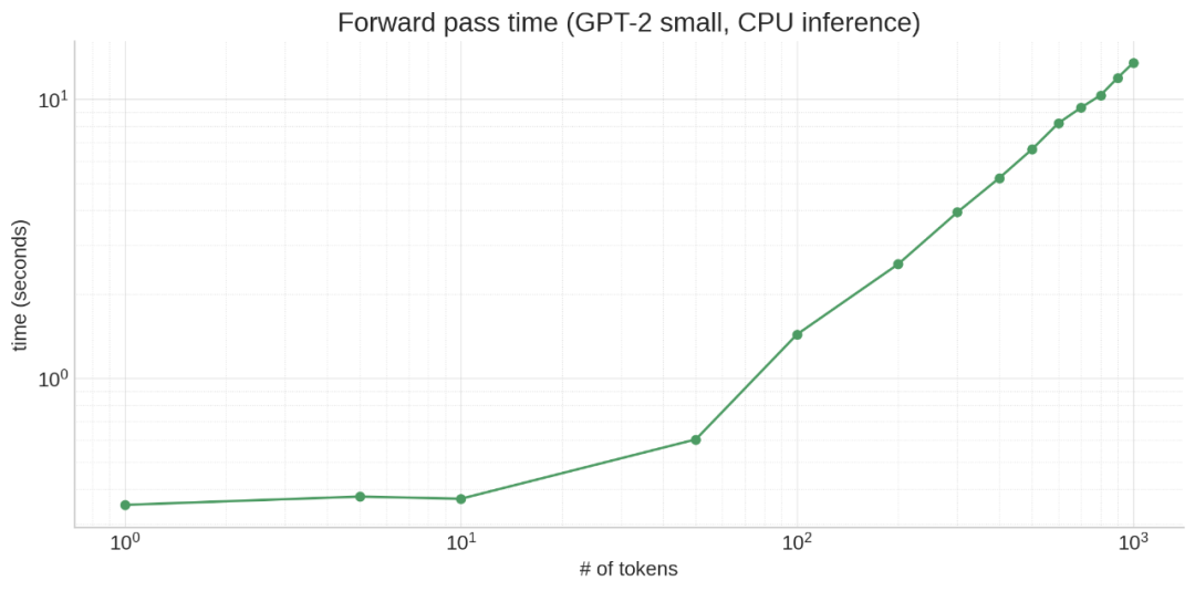
注意力(至少是普通注意力)也是一种二次算法:所有 token 都关注所有 token,导致 N^2 扩展,使一切变得更糟。
硬件原因是什么呢?很简单:LLM 规模很大。即使像 GPT-2 这样相对较小的模型也有 117M 参数,并且所有数据都必须存储在 RAM 中。
RAM 确实很慢,现代处理器(CPU 和 GPU)通过在靠近处理器的地方设置大量高速缓存(cache)来弥补这一点,从而使访问速度更快。
其细节根据处理器的类型和型号而有所不同,但关键是 LLM 权重不适合缓存,因此需要花费大量时间等待从 RAM 加载权重。
这会产生一些不直观的效果!例如,即使激活张量(tensor)大 10 倍,对 10 个 token 进行操作也不一定比对单个 token 进行操作慢很多,因为主要的时间消耗在于移动模型权重,而不是进行计算。
(1)指标
大模型推理速度“慢”到底是什么意思?
谈到 LLM 推理,人们采用的指标有很多:
-
Time to First Token(TtFT):收到 prompt 和返回第一个 token 之间需要多长时间?
-
生成延迟:收到 prompt 和返回最终 token 之间需要多长时间?
-
吞吐量
-
硬件利用:我们使用硬件的计算、内存带宽和其他功能的效率如何?
不同的优化对这些指标的影响不同。例如,批处理可以提高吞吐量并更好地利用硬件,但会增加 TtFT 和生成延迟。
02
硬件
加速推理的一个直接方法就是购买更好的硬件(通常是某种加速器:GPU 或 TPU),或者更好地利用您拥有的硬件。
使用加速器可以显著提高速度,但请记住,CPU 和加速器之间存在传输瓶颈。
如果模型不适合加速器的内存,则需要在整个前向传播过程中进行交换,这会大大减慢速度。
这也是 Apple M1/M2/M3 芯片在推理方面表现出色的原因之一,它们具有统一的 CPU 和 GPU 内存。
关于 CPU 和加速器推理,另一个关键是充分利用硬件,适当优化程序。
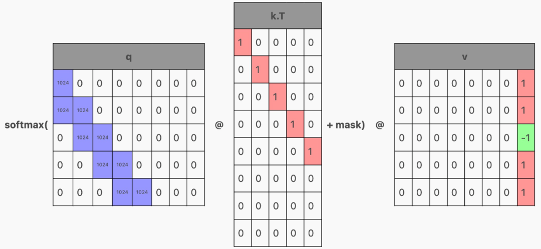
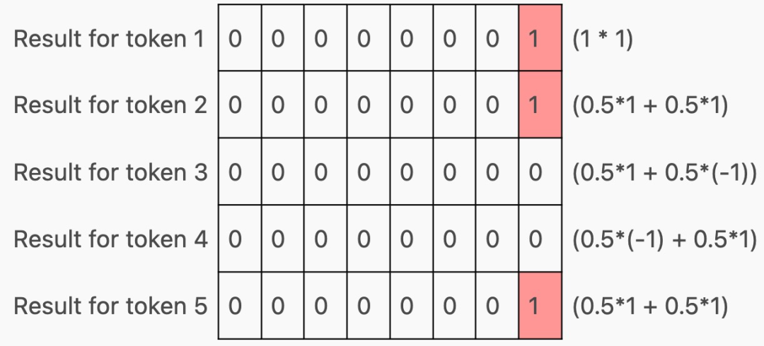
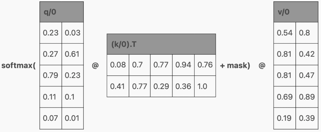
例如,在 PyTorch 中将注意力写入 F.softmax (q @ k.T/sqrt (k.size (-1)) + mask) @ v,能提供正确的结果。
但如果使用 torch.nn.function.scaled_dot_product_attention,会将计算委托给可用的 FlashAttention,这可以更好地利用缓存的手写内核产生 3 倍的加速。
(1)编译器
torch.compile、TinyGrad 和 ONNX 等编译器可以将简单的 Python 代码融合到针对硬件优化的内核中。
例如,我可以编写以下函数:
def foo(x):` `s = torch.sin(x)` `c = torch.cos(x)` `return s + c
简单来说,这个函数需要:
-
x.shape () 为 s 分配的内存
-
对 x 进行线性 scan 以计算每个元素的 sin
-
x.shape () 为 c 的另一种内存分配
-
线性 scan x 以计算每个元素的 cos
-
x.shape () 为结果张量分配的内存
-
线性 scan s 和 c,将它们添加到结果中
这些步骤每一个都很慢,并且某些步骤需要跨越 Python 和本机代码之间的界限。
如果我使用 torch.compile 编译这个函数会怎样?
>>> compiled_foo = torch.compile(foo, options={"trace.enabled": True, "trace.graph_diagram": True})``>>> # call with an arbitrary value to trigger JIT``>>> compiled_foo(torch.tensor(range(10)))``Writing FX graph to file: .../graph_diagram.svg``[2023-11-25 17:31:09,833] [6/0] torch._inductor.debug: [WARNING] model__24_inference_60 debug trace: /tmp/...zfa7e2jl.debug``tensor([ 1.0000, 1.3818, 0.4932, -0.8489, -1.4104, -0.6753, 0.6808, 1.4109,` `0.8439, -0.4990])
如果进入 debug 跟踪目录并打开其中的 output_code.py 文件,torch 就会为 CPU 生成一个优化的 C++ 内核,将 foo 融合到单个内核中。
如果使用 GPU 运行此程序,torch 将为 GPU 生成 CUDA 内核。
#include "/tmp/torchinductor_user/ib/cibrnuq56cxamjj4krp4zpjvsirbmlolpbnmomodzyd46huzhdw7.h"``extern "C" void kernel(const long* in_ptr0,` `float* out_ptr0)``{` `{` `#pragma GCC ivdep` `for(long i0=static_cast<long>(0L); i0<static_cast<long>(10L); i0+=static_cast<long>(1L))` `{` `auto tmp0 = in_ptr0[static_cast<long>(i0)];` `auto tmp1 = static_cast<float>(tmp0);` `auto tmp2 = std::sin(tmp1);` `auto tmp3 = std::cos(tmp1);` `auto tmp4 = tmp2 + tmp3;` `out_ptr0[static_cast<long>(i0)] = tmp4;` `}` `}``}
现在,步骤就变成了:
-
x.shape () 为结果张量分配的内存
-
对 x (in_ptr0) 进行线性扫描,计算 sin 和 cos 并将它们相加到结果中
对于大输入来说更简单、更快!
>>> x = torch.rand((10_000, 10_000))``>>> %timeit foo(x)``246 ms ± 8.89 ms per loop (mean ± std. dev. of 7 runs, 1 loop each)``>>> %timeit compiled_foo(x)``91.3 ms ± 14 ms per loop (mean ± std. dev. of 7 runs, 1 loop each)```# (for small inputs `compiled_foo` was actually slower--not sure why)`
请注意,torch.compile 将上面的代码专门用于传入 ((10,)) 的张量的特定大小。
如果我们传入许多不同大小的张量,torch.compile 将生成超过该大小的通用代码,但具有恒定大小可以使编译器在某些情况下生成更好的代码。
这是 torch.compile 的另一个函数:
>>> x = torch.rand((10_000, 10_000))``>>> %timeit foo(x)``246 ms ± 8.89 ms per loop (mean ± std. dev. of 7 runs, 1 loop each)``>>> %timeit compiled_foo(x)``91.3 ms ± 14 ms per loop (mean ± std. dev. of 7 runs, 1 loop each)```# (for small inputs `compiled_foo` was actually slower--not sure why)`
该函数具有数据相关的控制流,这意味着我们会根据变量的运行时值执行不同的操作。
如果以与编译 foo 相同的方式编译它,我们会得到两个图(因此有两个 debug 目录):
>>> compiled_gbreak = torch.compile(gbreak, options={"trace.enabled": True, "trace.graph_diagram": True})``>>> compiled_gbreak(torch.tensor(range(10)))``Writing FX graph to file: .../model__27_inference_63.9/graph_diagram.svg``[2023-11-25 17:59:32,823] [9/0] torch._inductor.debug: [WARNING] model__27_inference_63 debug trace: /tmp/torchinductor_user/p3/cp3the7mcowef7zjn7p5rugyrjdm6bhi36hf5fl4nqhqpfdqaczp.debug``Writing FX graph to file: .../graph_diagram.svg``[2023-11-25 17:59:34,815] [10/0] torch._inductor.debug: [WARNING] model__28_inference_64 debug trace: /tmp/torchinductor_user/nk/cnkikooz2z5sms2emkvwj5sml5ik67aqigynt7mp72k3muuvodlu.debug``tensor([ 1.0000, -0.1756, 2.6782, -0.7063, -2.5683, 2.7053, 0.9718, 0.5394,` `7.6436, -0.0467])
第一个内核实现了函数的 torch.sin (x) + torch.cos (x) 和 r.sum () < 0 部分:
#include "/tmp/torchinductor_user/ib/cibrnuq56cxamjj4krp4zpjvsirbmlolpbnmomodzyd46huzhdw7.h"``extern "C" void kernel(const long* in_ptr0,` `float* out_ptr0,` `float* out_ptr1,` `bool* out_ptr2)``{` `{` `{` `float tmp_acc0 = 0;` `for(long i0=static_cast<long>(0L); i0<static_cast<long>(10L); i0+=static_cast<long>(1L))` `{` `auto tmp0 = in_ptr0[static_cast<long>(i0)];` `auto tmp1 = static_cast<float>(tmp0);` `auto tmp2 = std::sin(tmp1);` `auto tmp3 = std::cos(tmp1);` `auto tmp4 = tmp2 + tmp3;` `out_ptr0[static_cast<long>(i0)] = tmp4;` `tmp_acc0 = tmp_acc0 + tmp4;` `}` `out_ptr1[static_cast<long>(0L)] = tmp_acc0;` `}` `}` `{` `auto tmp0 = out_ptr1[static_cast<long>(0L)];` `auto tmp1 = static_cast<float>(0.0);` `auto tmp2 = tmp0 < tmp1;` `out_ptr2[static_cast<long>(0L)] = tmp2;` `}``}
第二个内核实现了 return r - torch.tan (x) 分支:
#include "/tmp/torchinductor_user/ib/cibrnuq56cxamjj4krp4zpjvsirbmlolpbnmomodzyd46huzhdw7.h"``extern "C" void kernel(const float* in_ptr0,` `const long* in_ptr1,` `float* out_ptr0)``{` `{` `#pragma GCC ivdep` `for(long i0=static_cast<long>(0L); i0<static_cast<long>(10L); i0+=static_cast<long>(1L))` `{` `auto tmp0 = in_ptr0[static_cast<long>(i0)];` `auto tmp1 = in_ptr1[static_cast<long>(i0)];` `auto tmp2 = static_cast<float>(tmp1);` `auto tmp3 = std::cos(tmp2);` `auto tmp4 = tmp0 - tmp3;` `out_ptr0[static_cast<long>(i0)] = tmp4;` `}` `}``}
这就是所谓的「graph break」,这会让编译后的函数变慢,因为必须离开优化后的内核并返回到 Python 来评估分支。
最重要的是,另一个分支(return r + torch.tan (x))尚未编译,因为它尚未被采用。
这意味着它将在需要时动态编译,在不合适的时间(例如在服务用户请求的过程中)就会很糟糕。
理解 graph break 的一个方便工具是 torch._dynamo.explain:
# get an explanation for a given input``>>> explained = torch._dynamo.explain(gbreak)(torch.tensor(range(10)))`` ``# there's a break, because of a jump (if) on line 3``>>> explained.break_reasons``[GraphCompileReason(reason='generic_jump TensorVariable()', user_stack=[<FrameSummary file <stdin>, line 3 in gbreak>], graph_break=True)]`` ``# there are two graphs, since there's a break``>>> explained.graphs``[GraphModule(), GraphModule()]`` ``# let's see what each graph implements, without needing to dive into the kernels!``>>> for g in explained.graphs:``... g.graph.print_tabular()``... print()``...` `opcode name target args kwargs``------------- ------ ------------------------------------------------------ ------------ --------``placeholder l_x_ L_x_ () {}``call_function sin <built-in method sin of type object at 0x7fd57167aaa0> (l_x_,) {}``call_function cos <built-in method cos of type object at 0x7fd57167aaa0> (l_x_,) {}``call_function add <built-in function add> (sin, cos) {}``call_method sum_1 sum (add,) {}``call_function lt <built-in function lt> (sum_1, 0) {}``output output output ((add, lt),) {}`` ``opcode name target args kwargs``------------- ------ ------------------------------------------------------ ----------- --------``placeholder l_x_ L_x_ () {}``placeholder l_r_ L_r_ () {}``call_function tan <built-in method tan of type object at 0x7fd57167aaa0> (l_x_,) {}``call_function sub <built-in function sub> (l_r_, tan) {}``output output output ((sub,),) {}`` ``# pretty cool!
像 torch.compile 这样的工具是优化代码以获得更好的硬件性能,而无需使用 CUDA 编写内核。
03
批处理
在生成的未优化版本中,我们一次向模型传递一个序列,并在每一步要求它附加一个 token:
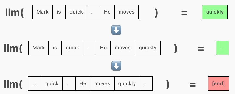
为了批量生成,我们一次向模型传递多个序列,在同一次前向传递中为每个序列生成一个补全。
这需要使用填充 token 在左侧或右侧将序列填充到相等的长度。填充 token(这里使用 [end])被隐藏在注意力掩码中,这样它们就不会影响生成。
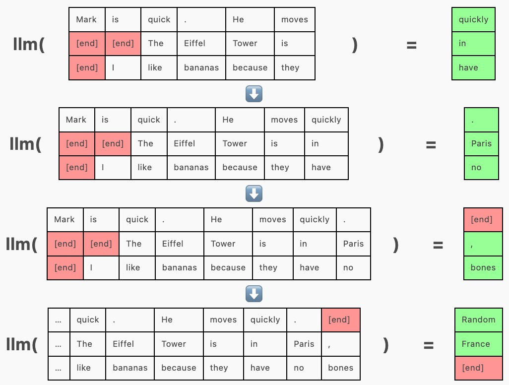
由于以这种方式批处理序列允许模型权重同时用于多个序列,因此一起运行整批序列比单独运行每个序列花费的时间更少。
例如,在我的机器上,使用 GPT-2 生成下一个 token:
-
20 tokens x 1 sequence = ~70ms
-
20 tokens x 5 sequences = ~220ms (线性扩展~350ms)
-
20 tokens x 10 sequences = ~400ms (线性扩展~700ms)
(1)连续批处理
在上面的示例中,「Mark is quick. He moves quickly.」在其他序列之前完成,但由于整个批次尚未完成,我们需要继续为其生成 token(“Random”)。
连续批处理通过在其他序列完成时在其 [end] token 之后将新序列插入批处理来解决此问题。

(2)缩小模型权重
浮点数有不同的大小,这对性能很重要。大多数情况下,对于常规软件,我们使用 64 位(双精度)IEEE 754 浮点,而 ML 传统上使用 32 位(单精度)IEEE 754:
>>> gpt2.transformer.h[0].attn.c_attn.weight.dtype``torch.float32
模型使用 fp32 进行良好的训练和推理,这为每个参数节省了 4 个字节 (50%),这个影响是巨大的,例如 7B 参数模型在 fp64 中将占用 56Gb,而在 fp32 中仅占用 28Gb。
训练和推理期间的大量时间都花在将数据从 RAM 移动到缓存和寄存器上,移动的数据越少越好。
fp16(或半精度)显然可以再节省 50%!这里有两个主要选项:fp16 和 bfloat16(brain float)。
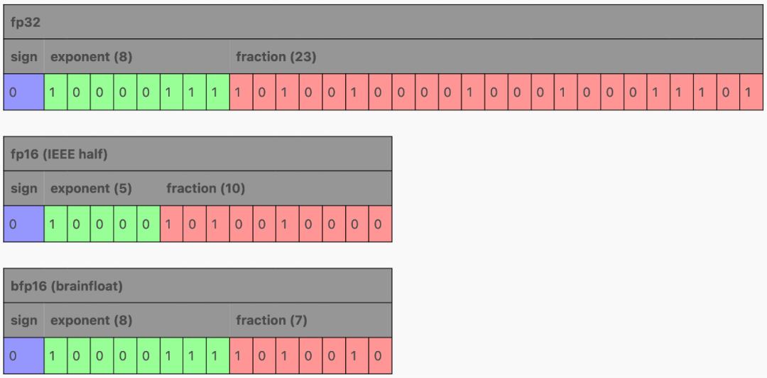
在减少 fp32 的字段时,fp16 和 bfloat16 进行了不同的权衡:fp16 试图通过缩小指数和分数字段来平衡范围和精度,而 bfloat16 通过保留 8 位指数来保留 fp32 的范围,同时将分数字段缩小到小于 fp16,损失了一些精度。
范围损失有时可能会成为 fp16 训练的问题,但对于推理来说,两者都可以,如果 GPU 不支持 bfloat16,fp16 可能是更好的选择。
还能更小吗?当然可以!
一种方法是量化以更大格式(例如 fp16)训练的模型。llama.cpp 项目(以及相关的 ML 库 ggml)定义了一整套量化格式。
这些量化的工作方式与 fp16 /bfloat16 略有不同 - 没有足够的空间来容纳整个数字,因此权重以块为单位进行量化,其中 fp16 充当块尺度(scale),然后量化块每个权重都乘以该尺度。
bitsandbytes 还为非 llama.cpp 项目实现了量化。
然而,使用更广泛的参数训练的模型量化越小,它就越有可能影响模型的性能,从而降低响应的质量。因此我们要尽可能少地采用量化,才能获得可接受的推理速度。
但我们也可以使用小于 fp16 的数据类型来微调或训练模型,例如使用 qLoRA 训练量化低阶适配器。
04
KV cache
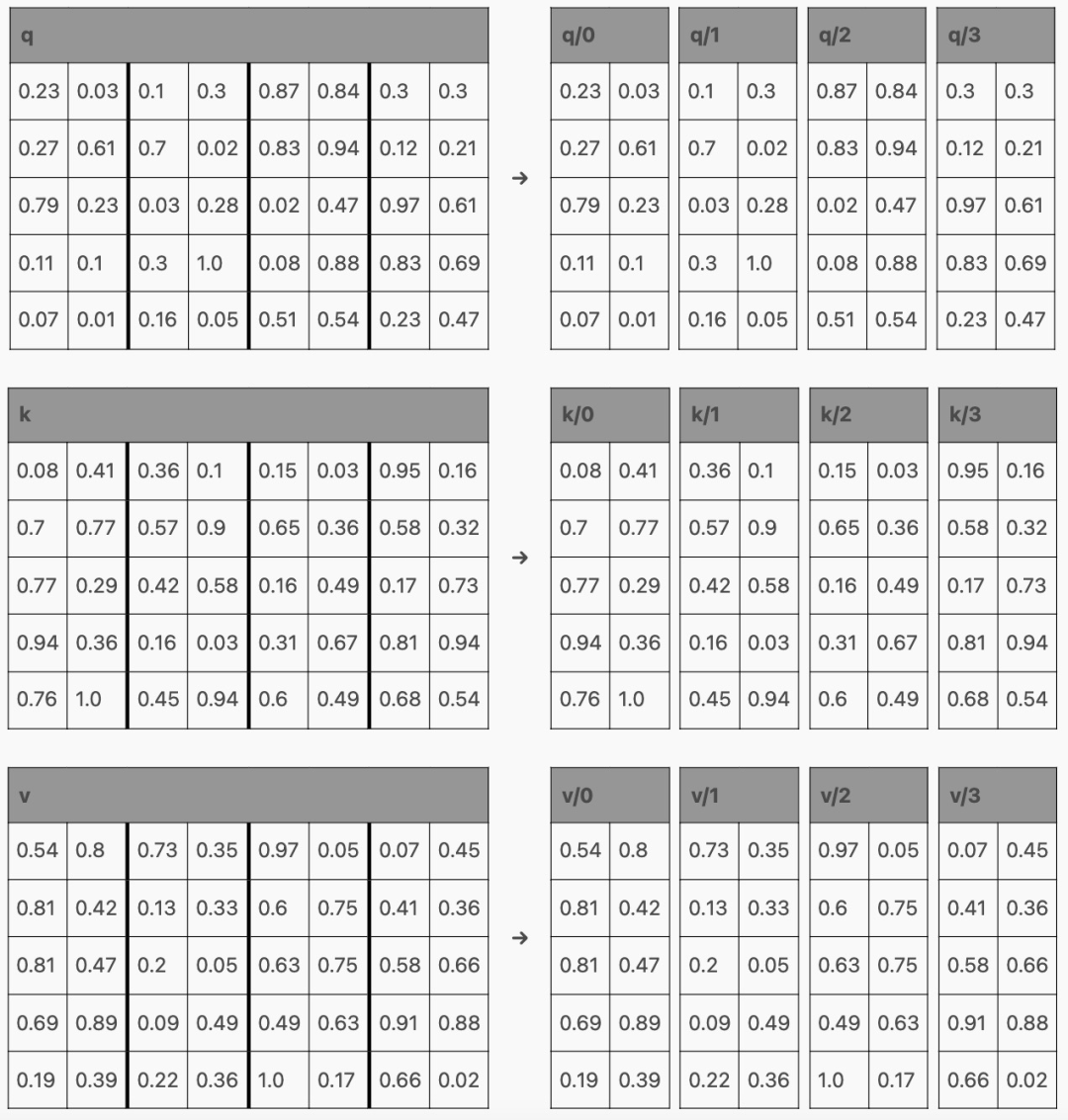
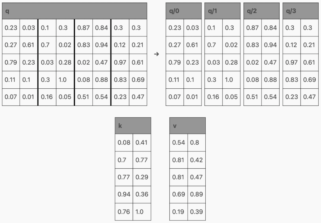
在 Transformer 内部,激活通过前馈层生成 qkv 矩阵,其中每一行对应一个 token:
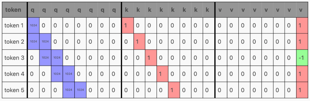
然后,qkv 矩阵被分割成 q、k 和 v,它们与注意力结合起来,如下所示:
以生成这样的矩阵:
现在,根据该层在 Transformer 中的位置,这些行可能会(在通过 MLP 之后)用作下一个 Transformer 块的输入,或者作为下一个 token 的预测,但请注意,每个 token 都有一行!
这是因为 Transformer 经过训练可以预测上下文窗口中每个 token 的下一个 token。
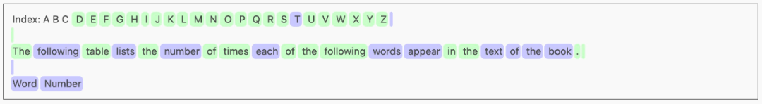
# the gpt2 tokenizer produces 3 tokens for this string``>>> tokens = tokenizer(" A B C").input_ids``>>> tokens``[317, 347, 327]`` ``# if we put that into the model, we get 3 rows of logits``>>> logits = gpt2(input_ids=torch.tensor(tokens)).logits.squeeze()``>>> logits.shape``torch.Size([3, 50257])`` ``# and if we argmax those, we see the model is predicting a next token``# for _every_ prompt token!``>>> for i, y in enumerate(logits.argmax(-1)):``... print(f"{tokenizer.decode(tokens[:i+1])!r} -> {tokenizer.decode(y)!r}")``' A' -> '.'``' A B' -> ' C'``' A B C' -> ' D'
在训练过程中,这种行为是可取的。这意味着更多的信息正在流入 Transformer,因为许多 token 都被评分。但通常在推理过程中,我们关心的只是底行,即最终 token 的预测。
我们如何才能从经过训练来预测整个上下文的 Transformer 中得到这一点呢?
让我们回到注意力的计算。如果 q 只有一行(对应于最后一个 token 的行)怎么办?
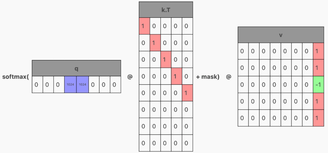
那么,这一行就将作为注意力结果,即最后一个 token 的结果。
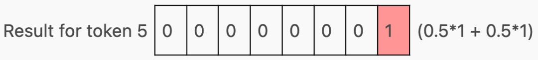
但只生成 q 的最后一行,意味着我们也只能在单行上运行生成 qkv 矩阵的层。那么 k 和 v 的其余行从哪里来?这就需要「KV 缓存(KV cache)」。
在模型内部,我们将注意力期间计算的 KV 值保存在每个 Transformer 块中。
然后在下一次生成时,只传入单个 token,并且缓存的 KV 行将堆叠在新 token 的 KV 行的顶部,以产生单行 Q 和多行 KV。
下面是使用 HuggingFace transformers API 进行 KV 缓存的示例,默认返回 KV cache 作为模型前向传递的一部分。
>>> tokens``[317, 347, 327] # the " A B C" string from before``>>> key_values = gpt2(input_ids=torch.tensor(tokens)).past_key_values``>>> tuple(tuple(x.shape for x in t) for t in key_values)``((torch.Size([1, 12, 3, 64]), torch.Size([1, 12, 3, 64])),` `(torch.Size([1, 12, 3, 64]), torch.Size([1, 12, 3, 64])),` `(torch.Size([1, 12, 3, 64]), torch.Size([1, 12, 3, 64])),` `(torch.Size([1, 12, 3, 64]), torch.Size([1, 12, 3, 64])),` `(torch.Size([1, 12, 3, 64]), torch.Size([1, 12, 3, 64])),` `(torch.Size([1, 12, 3, 64]), torch.Size([1, 12, 3, 64])),` `(torch.Size([1, 12, 3, 64]), torch.Size([1, 12, 3, 64])),` `(torch.Size([1, 12, 3, 64]), torch.Size([1, 12, 3, 64])),` `(torch.Size([1, 12, 3, 64]), torch.Size([1, 12, 3, 64])),` `(torch.Size([1, 12, 3, 64]), torch.Size([1, 12, 3, 64])),` `(torch.Size([1, 12, 3, 64]), torch.Size([1, 12, 3, 64])),` `(torch.Size([1, 12, 3, 64]), torch.Size([1, 12, 3, 64])))
KV cache 有助于解决 LLM 缓慢的问题,因为现在每个步骤中只传递一个 token,所以我们不必为每个新 token 重做所有事情。
然而,KV cache 的大小仍然每一步都会增长,从而减慢了注意力计算的速度。
KV cache 的大小也会带来自己的新问题,例如,对于 1000 个 token 的 KV cache,即使使用最小的 GPT-2,也会缓存 18432000 个值。如果每个值都是 fp32,那么单次生成的缓存几乎为 74MB。
对大模型来说,尤其是在需要处理许多并发客户端的服务器上运行的模型,KV cache 很快就会变得难以管理。
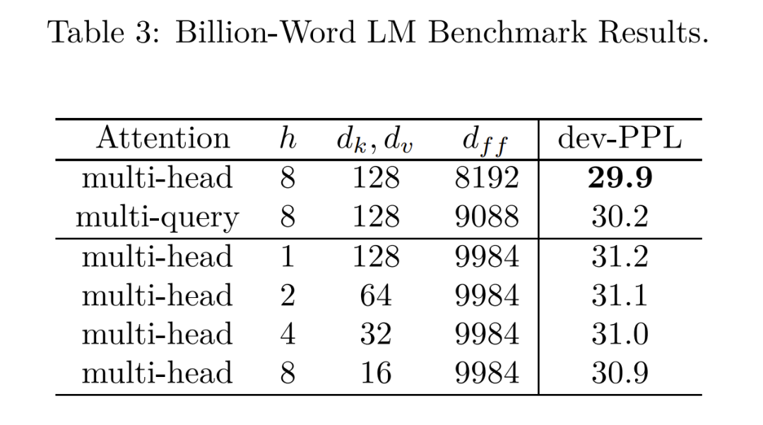
(1)多查询注意力
多查询注意力(Multi-Query Attention,MQA)是对模型架构的改变,通过为 Q 分配多个头,为 K 和 V 只分配一个头来缩小 KV 缓存的大小。
值得注意的是,使用 MQA 的模型比使用普通注意力训练的模型可以支持 KV 缓存中更多的 token。
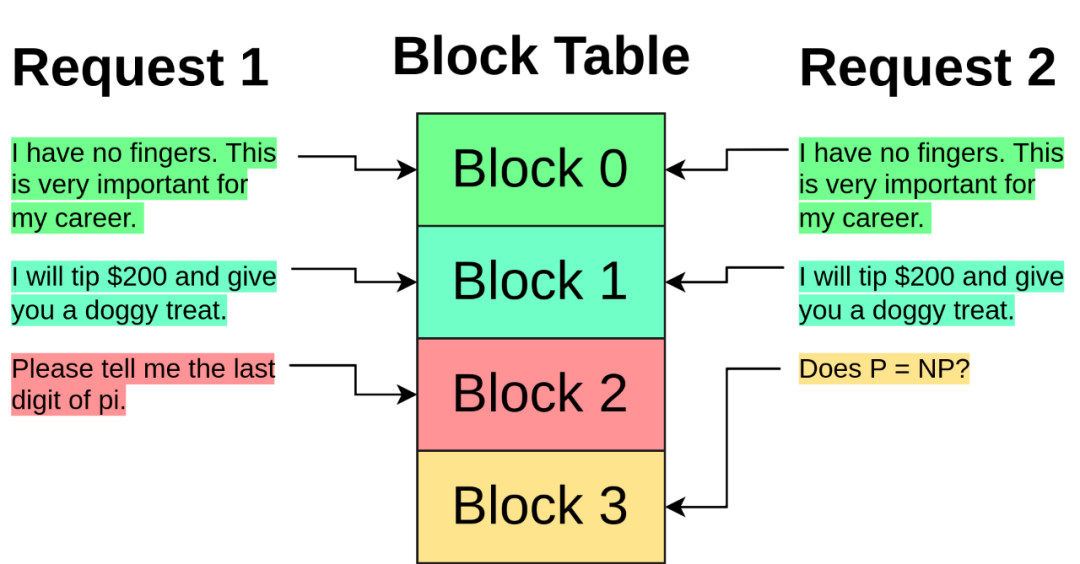
(2)分页注意力(PagedAttention)
大型 KV cache 的另一个问题是,它通常需要存储在连续的张量中,无论当前是否所有缓存都在使用。
这会导致多个问题:
-
需要预先分配比所需更多的空间
-
该保留空间不能被其他请求使用,即使还不需要它
-
具有相同前缀的请求不能共享该前缀的 KV 缓存
PagedAttention 从操作系统处理内存的方法中汲取灵感,解决了这些问题。
PagedAttention 会为请求分配一个块表(block table),类似于内存管理单元(MMU)。
每个请求没有与大量 KV 缓存项相关联,而是仅具有相对较小的块索引列表,类似于操作系统分页中的虚拟地址。这些索引指向存储在全局块表中的块。
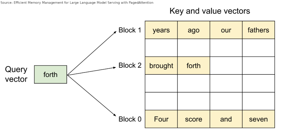
在注意力计算期间,PagedAttention 内核会遍历请求的块索引列表,并从全局块表中获取这些块,以便按照正确的顺序正常计算注意力。
05
猜测解码
要理解猜测解码,需要了解三件事。
首先,由于内存访问开销,模型运行少量 token 所需的时间与运行单个 token 大约相同:

其次,LLM 为上下文中的每个 token 生成预测:
>>> for i, y in enumerate(logits.argmax(-1)):``... print(f"{tokenizer.decode(tokens[:i+1])!r} -> {tokenizer.decode(y)!r}")``' A' -> '.'``' A B' -> ' C'``' A B C' -> ' D'
最后,有些词很容易预测。例如,在单词「going」之后,单词「to」极有可能是下一个 token。
def generate(prompt: str, tokens_to_generate: int) -> str:` `tokens: list[int] = tokenize(prompt)` `GOING, TO = tokenize(" going to")`` ` `for i in range(tokens_to_generate):` `if tokens[-1] == GOING:` `# do our speculative decoding trick` `logits = model.forward(tokens + [TO])` `# the token the model predicts will follow "... going"` `going_pred = argmax(logits[-2, :])` `# the token the model predicts will follow "... going to"`` to_pred = argmax(logits[-1, :])` `if going_pred == TO:` `# if our guess was correct, accept "to" and the next token after` `tokens += [TO, to_pred]` `else:` `# otherwise, accept the real next token` `# (e.g. "for" if the true generation was "going for broke")` `tokens += [going_pred]` `else:` `# do normal single-token generation` `logits = model.forward(tokens)` `tokens += [argmax(logits[-1])]`` ` `return detokenize(tokens)
我们只需要使用一个足够小的「draft 模型」(运行速度足够快),并使用相同的 tokenizer,以避免需要一遍又一遍地对序列进行 detokenize 和 retokenize。
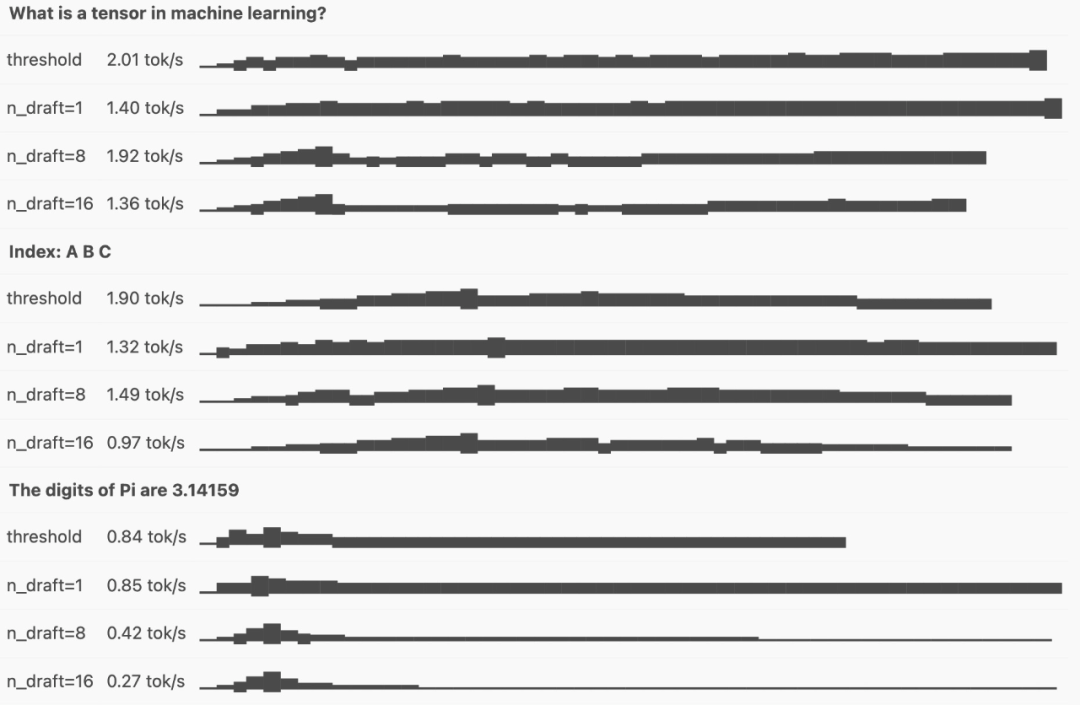
然而,猜测解码的性能可能非常依赖于上下文!如果 draft 模型与 oracle 模型相关性很好,并且文本很容易预测,那么您将获得大量 draft token 和快速推理。
但如果模型不相关,猜测解码实际上会使推理速度变慢,因为要浪费时间生成将被拒绝的 draft token。
def generate(prompt: str, tokens_to_generate: int, n_draft: int = 8) -> str:` `tokens: list[int] = tokenize(prompt)`` ` `for i in range(tokens_to_generate):` ``# generate `n_draft` draft tokens in the usual autoregressive way`` `draft = tokens[:]` `for _ in range(n_draft):` `logits = draft_model.forward(draft)` `draft.append(argmax(logits[-1]))`` ` `# run the draft tokens through the oracle model all at once` `logits = model.forward(draft)` `checked = logits[len(tokens) - 1 :].argmax(-1)`` ` `# find the index of the first draft/oracle mismatch—we'll accept every` `# token before it` `# (the index might be past the end of the draft, if every draft token` `# was correct)` `n_accepted = next(` `idx + 1` `for idx, (checked, draft) in enumerate(` `# we add None here because the oracle model generates one extra` `# token (the prediction for the last draft token)` `zip(checked, draft[len(tokens) :] + [None])` `)` `if checked != draft` `)` `tokens.extend(checked[:n_accepted])`` ` `return detokenize(tokens)


(1)阈值解码
一种缓解使用固定数量 draft token 问题的方法是「阈值解码」。
并不总是解码最大数量的 draft token,而是保留一个移动概率阈值,根据当前的 token 数量进行校准。draft token 会一直生成,直到 draft 的累积概率低于此阈值。
例如,如果阈值是 0.5,并且我们以 0.75 的概率生成 draft token「the」,继续下去。
如果下一个 token「next」的概率为 0.5,则累积概率 0.375 将低于阈值,因此会停止生成并将两个 draft token 提交给 oracle 模型。
然后,根据 draft 被接受的程度,向上或向下调整阈值,以尝试用实际接受率来校准 draft 模型的置信度。
def speculative_threshold(` `prompt: str,` `max_draft: int = 16,` `threshold: float = 0.4,` `threshold_all_correct_boost: float = 0.1,``):` `tokens = encoder.encode(prompt)`` ` ``# homegrown KV cache setup has an `n_tokens` method that returns the length`` ``# of the cached sequence, and a `truncate` method to truncate that sequence`` `# to a specific token` `model_kv = gpt2.KVCache()` `draft_kv = gpt2.KVCache()`` ` `while True:` ``# generate up to `max_draft` draft tokens autoregressively, stopping`` `` # early if we fall below `threshold` `` `draft = tokens[:]` `drafted_probs = []` `for _ in range(max_draft):` `logits = draft_model.forward(draft[draft_kv.n_tokens() :], draft_kv)` `next_id = np.argmax(logits[-1])` `next_prob = gpt2.softmax(logits[-1])[next_id]` `if not len(drafted_probs):` `drafted_probs.append(next_prob)` `else:` `drafted_probs.append(next_prob * drafted_probs[-1])` `draft.append(int(next_id))` `if drafted_probs[-1] < threshold:` `break` `n_draft = len(draft) - len(tokens)`` ` `# run draft tokens through the oracle model` `logits = model.forward(draft[model_kv.n_tokens() :], model_kv)` `checked = logits[-n_draft - 1 :].argmax(-1)` `n_accepted = next(` `idx + 1` `for idx, (checked, draft) in enumerate(` `zip(checked, draft[len(tokens) :] + [None])` `)` `if checked != draft` `)` `yield from checked[:n_accepted]` `tokens.extend(checked[:n_accepted])`` ` `if n_accepted <= n_draft:` `# adjust threshold towards prob of last accepted token, if we` `# ignored any draft tokens` `threshold = (threshold + drafted_probs[n_accepted - 1]) / 2` `else:` `# otherwise, lower the threshold slightly, we're probably being` `# too conservative` `threshold -= threshold_all_correct_boost` `# clamp to avoid pathological thresholds` `threshold = min(max(threshold, 0.05), 0.95)`` ` `# don't include oracle token in kv cache` `model_kv.truncate(len(tokens) - 1)` `draft_kv.truncate(len(tokens) - 1)
此外,分阶段猜测解码为普通猜测解码添加了一些改进。
(2)指导型生成
语法指导型生成可约束模型的输出遵循某些语法,从而提供保证匹配某些语法(例如 JSON)的输出。这对模型推理的可靠性和速度都有益。
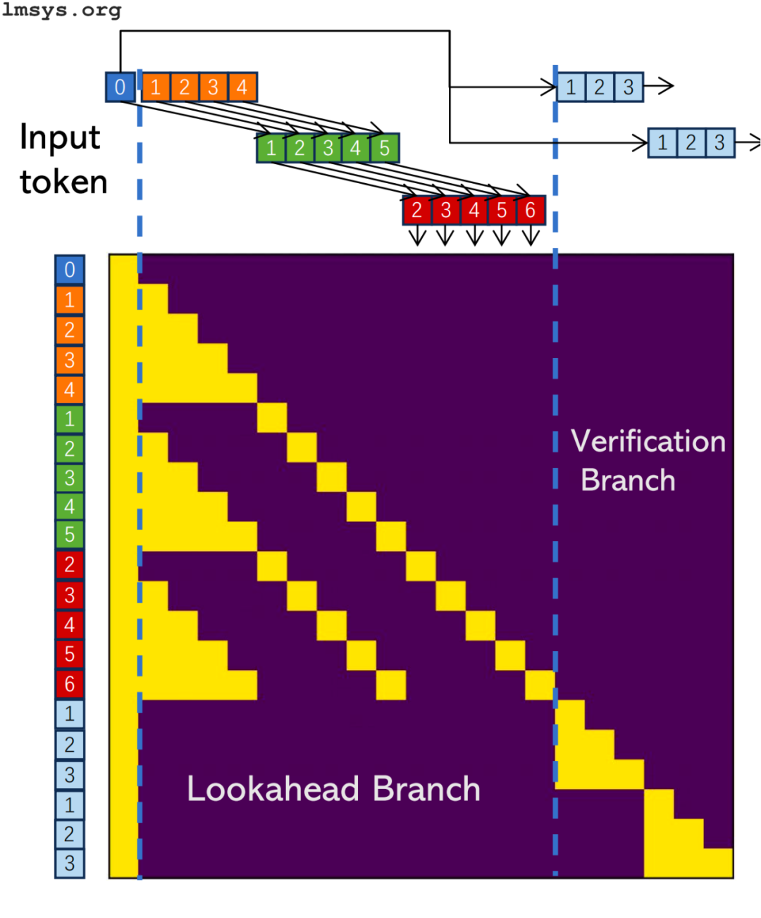
(3)前向解码
前向解码是一种新的猜测解码方法,不需要 draft 模型。相反,模型本身用于两个分支:预测和扩展候选 N-gram 的前向分支和验证候选的验证分支。
前向分支类似于常规猜测解码中的 draft 模型,而验证分支与 oracle 模型具有相同的作用。
还有一种方法是 prompt 查找解码,其中 draft 模型被上下文中的简单字符串匹配所取代。
最后,作者从稀疏注意力(sparse attention)和非 Transformer 架构两个方面简单阐述了训练时间优化的方法。
END
那么,如何系统的去学习大模型LLM?
我在一线互联网企业工作十余年里,指导过不少同行后辈。帮助很多人得到了学习和成长。
作为一名热心肠的互联网老兵,我意识到有很多经验和知识值得分享给大家,也可以通过我们的能力和经验解答大家在人工智能学习中的很多困惑,所以在工作繁忙的情况下还是坚持各种整理和分享。
但苦于知识传播途径有限,很多互联网行业朋友无法获得正确的资料得到学习提升,故此将并将重要的AI大模型资料包括AI大模型入门学习思维导图、精品AI大模型学习书籍手册、视频教程、实战学习等录播视频免费分享出来。
所有资料 ⚡️ ,朋友们如果有需要全套 《LLM大模型入门+进阶学习资源包》,扫码获取~
篇幅有限,部分资料如下:
👉LLM大模型学习指南+路线汇总👈
💥大模型入门要点,扫盲必看!

💥既然要系统的学习大模型,那么学习路线是必不可少的,这份路线能帮助你快速梳理知识,形成自己的体系。
路线图很大就不一一展示了 (文末领取)

👉大模型入门实战训练👈
💥光学理论是没用的,要学会跟着一起做,要动手实操,才能将自己的所学运用到实际当中去,这时候可以搞点实战案例来学习。

👉国内企业大模型落地应用案例👈
💥两本《中国大模型落地应用案例集》 收录了近两年151个优秀的大模型落地应用案例,这些案例覆盖了金融、医疗、教育、交通、制造等众多领域,无论是对于大模型技术的研究者,还是对于希望了解大模型技术在实际业务中如何应用的业内人士,都具有很高的参考价值。 (文末领取)

👉GitHub海量高星开源项目👈
💥收集整理了海量的开源项目,地址、代码、文档等等全都下载共享给大家一起学习!

👉LLM大模型学习视频👈
💥观看零基础学习书籍和视频,看书籍和视频学习是最快捷也是最有效果的方式,跟着视频中老师的思路,从基础到深入,还是很容易入门的。 (文末领取)

👉640份大模型行业报告(持续更新)👈
💥包含640份报告的合集,涵盖了AI大模型的理论研究、技术实现、行业应用等多个方面。无论您是科研人员、工程师,还是对AI大模型感兴趣的爱好者,这套报告合集都将为您提供宝贵的信息和启示。

👉获取方式:
这份完整版的大模型 LLM 学习资料已经上传CSDN,朋友们如果需要可以微信扫描下方CSDN官方认证二维码免费领取【保证100%免费】
😝有需要的小伙伴,可以Vx扫描下方二维码免费领取🆓


 7267
7267

 被折叠的 条评论
为什么被折叠?
被折叠的 条评论
为什么被折叠?
 到【灌水乐园】发言


