3DGS基础初了解（二）

上篇博客主要介绍了Radiance Field辐射场和Rendering，最后还进行了NeRF和3DGS的对比，详情请看3DGS基础初了解（一）

本篇博客将重点介绍3DGS的一些原理性内容（不涉及具体原理推导和代码）

参考论文A Survey on 3D Gaussian Splatting

1 Basic

1.1 3DGS突破点

简而言之：在不依赖深度神经网络的情况下，实现实时、高分辨率的图像渲染

1.2 properties

• center (position) μ —— 位置
• 3D covariance matrix Σ —— 协方差矩阵 →决定形状和方向
• opacity α —— 不透明度 →所有属性都可以通过后传播来学习和优化
• color c —— 颜色 →由球形谐波来表示，依赖视图外观

2 Rendering

• objective目的 : generate an image from a specified camera pose

我在学习的时候是将NeRF与3DGS进行对比来理解3DGS到底“优”在何处，所以下面也将从NeRF开始

• NeRf : computationally demanding volumetric ray-marching , sampling 3D space points per pixel
• NeRF的drawback : high-resolution image systhesis fail to achieve real-time rendering, especially for platforms with limited computing resources

在了解3DGS具体是如何进行Rendering之前我先介绍几个基础的概念

• 前向映射(forward mapping)：3D对象的每个点直接映射到2D屏幕空间，也就是光栅化(rasterization）
• 反向映射(backward mapping)：从2D屏幕的像素出发，反向追踪到3D场景中的点，比如射线追踪(ray tracing)
• 体素渲染：沿着射线积分颜色和透明度，需要累积每个采样点的贡献
• splatting : 将3D点或者小体素投影到2D，形成覆盖区域的点或形状，然后混合颜色

接下来看图理解

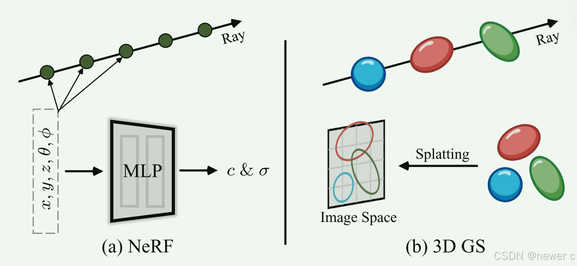
• NeRF 是如何得到最终像素的颜色呢？
  → 反向映射(Ray tracing)——NeRF对每个像素，发射一条射线到场景中，沿着射线采样多个点，每个点通过MLP计算出颜色和密度，然后通过体素渲染（volume rendering）将这些采样点的结果累积起来，得到最终像素的颜色
• 3DGS是如何得到最终像素的颜色呢？
  → 前向映射(Rasterization) → 颜色混合

前向映射的核心流程：
（1）Splatting : 3D高斯→椭圆

• 1️⃣将3D高斯从世界坐标转换为相机坐标
• 2️⃣splatting these Gaussians into 2D image place via an approximation of the projective transformation(投影变换)

计算表征投影的2D高斯的2D协方差矩阵∑’：其中，∑是3D协方差矩阵，描述了3DGS的空间分布；W是转换矩阵；J是投影变换的雅可比矩阵，描述局部线性近似
$${\Sigma }^{\prime }=JW\Sigma W^T{J}^T$$

• 3️⃣Rendering by Pixels : 给定像素的位置，通过视角变换矩阵W计算与所有重叠高斯的距离，形成排序表N，然后使用Alpha混合得到最终的颜色。

我初读这句话的时候每个字都认识但是连在一起就不知道讲什么，所以下面是我拆解这句话的解释（有点啰啰嗦嗦的，可以直接跳过）

• “通过视角变换矩阵W计算与所有重叠高斯的距离” : 通过视角变换矩阵W，把每个3D高斯的位置转换成相机视角下的目标，得到他们到相机的深度（即距离）。讲人话就是：把3D场景里的物体位置转换成**“距离相机多远”**的数据
• 怎么“形成排序表N”？ 把所有覆盖这个像素的高斯按距离排序，生成一个由近到远（或由远到近）的列表（N）

下面的公式是权重的计算：权重表示该高斯对当前像素的颜色贡献强度，随距离高斯中心越远而指数衰减。
$${\alpha }_n^{\prime }={\alpha }_n\times exp(-\frac{1}{2}({\mathbf{x}}^{\prime }-{\mu }_n^{\prime }{)}^T{\Sigma }_n^{\prime -1}({\mathbf{x}}^{\prime }-{\mu }_n^{\prime }))$$
在上面的公式中，x’_n和μ’_n是投影空间中的坐标

• 使用Alpha混合怎么算颜色？从最远的高斯开始逐个叠加颜色，同时考虑它们的透明度（越透明的高斯对最终的颜色影响越小）

下面的公式进行颜色混合的计算：
$$C=\sum _{n=1}^{|\mathcal{N}|}{c}_n{\alpha }_n^{\prime }\prod _{j=1}^{n-1}\left(1-{\alpha }_j^{\prime }\right)$$
在上面公式中连乘项表示将所有前面高斯的“未被遮挡比例”（1-w_j）连乘，得到当前高斯能“透过”高斯的剩余可见性。
讲的通俗易懂就是：当计算后面高斯的颜色贡献时，必须考虑前面高斯的不透明度，因为前面高斯可能部分遮挡后面高斯。如果前面高斯的α值高，那么后面高斯的可见部分就会减少。

Parallel Rendering 并行渲染

避免为每个像素推导高斯分布的成本计算，3DGS将精度由像素级转移到面片级细节(from pixel-level to patch-level detail)
下图引用自论文A Survey on 3D Gaussian Splatting，该图完整地展现了整个forward process

• （a）splatting过程，详细解析可会看前面
• （b）divides the image into multiple non-overlapping patches：每个3D高斯投影到屏幕后，会覆盖一定的像素区域（椭圆泼溅）。根据其覆盖的像素范围，将高斯分配到可能重叠的图块中。
• （c）3D GS replicates the Gaussians which cover several tiles, assigning each copy an identifier, i.e., a tile ID.
• （d）By rendering the sorted Gaussians, we can obtain all pixels within the tile. Note that the computational workflows for pixels and tiles are independent and can be done in parallel.

按照我的理解（啰哩吧嗦）：3D Gaussians是一个个小椭球，Image Space相当于是墙，将一个个椭球往墙上扔，留下的痕迹就是图（b）中的左边的小图，然后将墙面切割成4个Tiles，接着就知道每个椭球会分别在哪几个Tiles中，罗列出来就是图（c）中的左边。因为我的处理是处理Tiles，所以根据深度的顺序将同一个Tile的“ID Card”（我将一个标有Tile X : Depth的方框理解为一个“ID Card”）进行整理排序可以得到图（c）中的“Sorted 2D Gaussians”。然后对一个Tile内的每个像素进行并行计算颜色（Parallel Rendering），最后将所有处理完的结果合并就形成完整图像。（如果该理解有错误，请各位佬评论区指正🫡）

这里最精彩的部分就是并行处理：

• 图块级并行：每个图块独立处理：不同图块的计算流程互不依赖，GPU可以同时处理多个图块（如同时处理图块A、B、C）
• 像素级并行：每个像素独立计算：在一个图块内的所有高斯按深度排序后形成一个列表，但排序过程仅在局部进行（不影响其他图块）
• 高斯排序的并行优化：每个图块内的所有高斯按深度排序后形成一个列表

3 Optimization

3DGS的核心：lies an optimization procedure devised to construct a copious collection of 3D Gaussians 旨在构建大量的3D高斯集合的优化程序

• 如何进行Parameter Optimization
• Loss Function : be optimized by stochastic gradient descent（随机梯度下降） using the ℓ1 and D-SSIM loss functions (λ ∈ [0, 1] is a weighting factor)
  $$\mathcal{L}=(1-\lambda ){\mathcal{L}}_1+\lambda {\mathcal{L}}_{\mathrm{D}-\mathrm{SSIM}}$$
• Parameter Update : Most properties of a 3D Gaussian can be optimized directly through back-propagation
• 补充：directly optimize the covariance matrix ∑ can result in a non-positive semi-definite matrix -> in order to circumvent this issue : 3DGS optimize a quaternion q(rotation) and a 3D vector s(scale)——这种方法将协方差矩阵∑重建如下：where R is the rotation matrix derived from the quaternion q, and S is the scaling matrix given by diag(s)
  $$\Sigma =RS{S}^T{R}^T$$
• To avoid the cost of automatic differentiation, 3D GS derives the gradients for q and s so as to compute them directly during optimization

4 Density Control

4.1 Initialization

• starts with the initial set of sparse points from SfM or random initialization
• 初始化对于convergence and reconstruction quality很重要
• control the density of 3D Gaussians : point densification and pruning（下面将会重点介绍）

4.2 Point Densification

• adaptively increase the density of Gaussians to better capture the details of a scene
• focuses on areas with missing geometric features or regions where Gaussians are too spread out
• It involves either cloning small Gaussians in under-reconstructed areas or splitting large Gaussians in over-reconstructed regions（相当于缺就补，超就减）
• be performed at regular intervals —— focusing on those Gaussians with large view-space positional gradients (i.e., above a specific thresh-old)
• 目的：寻求高斯在3D空间中的最佳分布和表示，提高整体重建的整体质量

4.3 Point Pruning

• regularization process : involves the removal of superfluous or less impactdul Gaussians
• eliminating Gaussians that are virtually transparent (with α below a specified threshold) and those that are excessively large in either world-space or view-space
• prevent unjustified increases in Gaussian density near input cameras : the alpha value of the Gaussian is set close to zero often a certain number of iterations
• 目的：control the density of Gaussians，节省计算资源，确保模型中的高斯模型对场景的表示保持精确有效