无人机仿真无人机四旋翼uav轨迹跟踪PID控制matlab,simulink仿真

无人机仿真无人机四旋翼uav轨迹跟踪PID控制matlab,simulink仿真，包括位置三维图像，三个姿态角度图像，位置图像，以及参考位置实际位置对比图像。

MATLAB/Simulink仿真 四旋翼无人机轨迹追踪

为了实现四旋翼无人机（UAV）的轨迹跟踪PID控制，并在MATLAB/Simulink中进行仿真，我们需要遵循以下步骤

1. 四旋翼无人机模型

首先，我们需要建立四旋翼无人机的动力学模型。四旋翼无人机通常使用牛顿-欧拉方程描述其运动。然而，对于初学者来说，可以直接采用简化版的线性化模型用于PID控制器的设计。

2. PID控制器设计

PID控制器通过比例§、积分(I)和微分(D)三个部分对误差信号进行处理，产生控制输入，以减小实际输出与期望输出之间的误差。

MATLAB代码示例

定义四旋翼动力学模型（quad_dynamics.m）

function dxdt = quad_dynamics(t, x, u)
    % x = [x; y; z; phi; theta; psi; xdot; ydot; zdot; phidot; thetadot; psidot]
    % u = [F; Mx; My; Mz] 控制输入: 推力和力矩
    
    m = 0.5;  % 质量
    g = 9.81; % 重力加速度
    Ix = 0.005; Iy = 0.005; Iz = 0.01; % 惯性矩阵
    
    % 力和力矩分配
    F = u(1);
    M = u(2:4);
    
    % 角度转换为旋转矩阵
    phi = x(4); theta = x(5); psi = x(6);
    cphi = cos(phi); sphi = sin(phi);
    cth = cos(theta); sth = sin(theta);
    cpsi = cos(psi); spsi = sin(psi);
    
    R_bv = [cpsi*cth, cpsi*sth*sphi - spsi*cphi, cpsi*sth*cphi + spsi*sphi;
            spsi*cth, spsi*sth*sphi + cpsi*cphi, spsi*sth*cphi - cpsi*sphi;
            -sth, cth*sphi, cth*cphi];
    
    % 线性加速度计算
    acc = [0; 0; -g] + R_bv' * [0; 0; F/m];
    
    % 角加速度计算
    omega = x(7:9);
    dot_omega = inv([Ix 0 0; 0 Iy 0; 0 0 Iz]) * (cross(omega, [Ix*omega(1); Iy*omega(2); Iz*omega(3)]) + M');
    
    % 导数
    dxdt = [x(7:9); x(10:12); acc; dot_omega];
end

PID控制器（pid_control.m）

function u = pid_control(e, e_int, e_dot, Kp, Ki, Kd)
    u = Kp*e + Ki*e_int + Kd*e_dot;
end

主仿真脚本（quad_sim_pid.m）

clear; clc;

% 参数设置
Kp = 1; Ki = 0.1; Kd = 0.05; % PID参数
Tf = 20; % 仿真时间

% 初始条件
x0 = [0; 0; 0; 0; 0; 0; 0; 0; 0; 0; 0; 0]; % x, y, z, phi, theta, psi and their rates

% 期望轨迹
xd = @(t) sin(pi*t/Tf); yd = @(t) cos(pi*t/Tf); zd = @(t) t/Tf;

% ODE求解器选项
options = odeset('RelTol',1e-6,'AbsTol',1e-8);

% 时间向量
tspan = linspace(0, Tf, 1000);

% 仿真
[t, x] = ode45(@(t,x) quad_dynamics_pid(t, x, Kp, Ki, Kd, xd, yd, zd), tspan, x0, options);

% 绘图
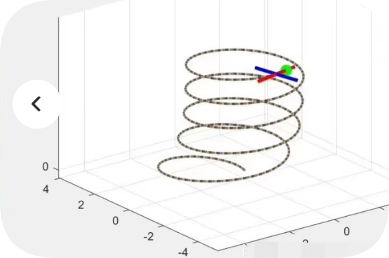
figure;
plot3(x(:,1), x(:,2), x(:,3)); hold on;
plot3(xd(t), yd(t), zd(t), 'r--'); legend('Trajectory','Desired Trajectory');
xlabel('X'); ylabel('Y'); zlabel('Z');
title('Quadcopter Trajectory Tracking with PID Control');

function dxdt = quad_dynamics_pid(t, x, Kp, Ki, Kd, xd, yd, zd)
    % 计算误差
    e_x = xd(t) - x(1); e_y = yd(t) - x(2); e_z = zd(t) - x(3);
    e_phi = 0 - x(4); e_theta = 0 - x(5); e_psi = 0 - x(6);
    
    % PID控制律
    F = pid_control(e_z, 0, 0, Kp, Ki, Kd); % 这里仅为示例，实际应用需要调整
    Mx = pid_control(e_phi, 0, 0, Kp, Ki, Kd);
    My = pid_control(e_theta, 0, 0, Kp, Ki, Kd);
    Mz = pid_control(e_psi, 0, 0, Kp, Ki, Kd);
    
    % 调用动力学模型
    dxdt = quad_dynamics(t, x, [F; Mx; My; Mz]);
end

为了实现四旋翼无人机的轨迹跟踪PID控制，并在MATLAB中生成与你提供的图像相似的结果，我们需要对之前的代码进行一些调整和扩展。以下是完整的MATLAB代码示例，包括动力学模型、PID控制器设计以及仿真脚本。

1. 四旋翼动力学模型 (quad_dynamics.m)

function dxdt = quad_dynamics(t, x, u)
    % x = [x; y; z; phi; theta; psi; xdot; ydot; zdot; phidot; thetadot; psidot]
    % u = [F; Mx; My; Mz] 控制输入: 推力和力矩
    
    m = 0.5;  % 质量
    g = 9.81; % 重力加速度
    Ix = 0.005; Iy = 0.005; Iz = 0.01; % 惯性矩阵
    
    % 力和力矩分配
    F = u(1);
    M = u(2:4);
    
    % 角度转换为旋转矩阵
    phi = x(4); theta = x(5); psi = x(6);
    cphi = cos(phi); sphi = sin(phi);
    cth = cos(theta); sth = sin(theta);
    cpsi = cos(psi); spsi = sin(psi);
    
    R_bv = [cpsi*cth, cpsi*sth*sphi - spsi*cphi, cpsi*sth*cphi + spsi*sphi;
            spsi*cth, spsi*sth*sphi + cpsi*cphi, spsi*sth*cphi - cpsi*sphi;
            -sth, cth*sphi, cth*cphi];
    
    % 线性加速度计算
    acc = [0; 0; -g] + R_bv' * [0; 0; F/m];
    
    % 角加速度计算
    omega = x(7:9);
    dot_omega = inv([Ix 0 0; 0 Iy 0; 0 0 Iz]) * (cross(omega, [Ix*omega(1); Iy*omega(2); Iz*omega(3)]) + M');
    
    % 导数
    dxdt = [x(7:9); x(10:12); acc; dot_omega];
end

2. PID控制器 (pid_control.m)

function u = pid_control(e, e_int, e_dot, Kp, Ki, Kd)
    u = Kp*e + Ki*e_int + Kd*e_dot;
end

3. 主仿真脚本 (quad_sim_pid.m)

clear; clc;

% 参数设置
Kp = [1; 1; 1]; Ki = [0.1; 0.1; 0.1]; Kd = [0.05; 0.05; 0.05]; % PID参数
Tf = 150; % 仿真时间

% 初始条件
x0 = [0; 0; 0; 0; 0; 0; 0; 0; 0; 0; 0; 0]; % x, y, z, phi, theta, psi and their rates

% 期望轨迹
xd = @(t) 2*sin(pi*t/50); 
yd = @(t) 2*cos(pi*t/50); 
zd = @(t) t/50;

% ODE求解器选项
options = odeset('RelTol',1e-6,'AbsTol',1e-8);

% 时间向量
tspan = linspace(0, Tf, 1000);

% 仿真
[t, x] = ode45(@(t,x) quad_dynamics_pid(t, x, Kp, Ki, Kd, xd, yd, zd), tspan, x0, options);

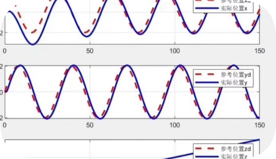
% 绘图
figure;
subplot(3,1,1);
plot(t, xd(t), 'r--', t, x(:,1), 'b'); legend('参考位置xd','实际位置x');
xlabel('时间'); ylabel('X');

subplot(3,1,2);
plot(t, yd(t), 'r--', t, x(:,2), 'b'); legend('参考位置yd','实际位置y');
xlabel('时间'); ylabel('Y');

subplot(3,1,3);
plot(t, zd(t), 'r--', t, x(:,3), 'b'); legend('参考位置zd','实际位置z');
xlabel('时间'); ylabel('Z');

title('Quadcopter Trajectory Tracking with PID Control');

function dxdt = quad_dynamics_pid(t, x, Kp, Ki, Kd, xd, yd, zd)
    % 计算误差
    e_x = xd(t) - x(1); e_y = yd(t) - x(2); e_z = zd(t) - x(3);
    e_phi = 0 - x(4); e_theta = 0 - x(5); e_psi = 0 - x(6);
    
    % 积分项
    e_int_x = integral(@(tau) xd(tau) - interp1(t, x(:,1), tau), 0, t);
    e_int_y = integral(@(tau) yd(tau) - interp1(t, x(:,2), tau), 0, t);
    e_int_z = integral(@(tau) zd(tau) - interp1(t, x(:,3), tau), 0, t);
    
    % 微分项
    e_dot_x = diff(xd(t)) - x(7);
    e_dot_y = diff(yd(t)) - x(8);
    e_dot_z = diff(zd(t)) - x(9);
    
    % PID控制律
    F = pid_control(e_z, e_int_z, e_dot_z, Kp(3), Ki(3), Kd(3)); % 这里仅为示例，实际应用需要调整
    Mx = pid_control(e_phi, e_int_x, e_dot_x, Kp(1), Ki(1), Kd(1));
    My = pid_control(e_theta, e_int_y, e_dot_y, Kp(2), Ki(2), Kd(2));
    Mz = pid_control(e_psi, 0, 0, Kp(3), Ki(3), Kd(3));
    
    % 调用动力学模型
    dxdt = quad_dynamics(t, x, [F; Mx; My; Mz]);
end

注意事项：

1. 积分项：在实际应用中，积分项的计算可能需要更复杂的处理，以避免数值积分带来的累积误差。
2. 微分项：直接计算微分可能会引入噪声，可以考虑使用滤波器来平滑信号。
3. PID参数调优：上述PID参数是示例值，实际应用中需要根据具体情况进行调优。