基于车辆运动学模型的LQR横向控制算法

一，车辆运动学模型的建立

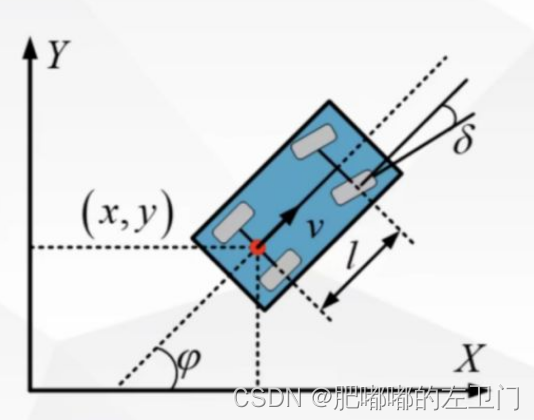
 如图所示，对于横向控制而言，因变量为，自变量为

将速度沿轴分解得车辆的模型为：

即：

其中，因为是横向控制，故假设是常数

上述车辆运动学模型为非线性模型：

二，车辆运动学模型的线性化：泰勒展开

在参考点处的泰勒展开公式,忽略高次项为：

其中，

令,

则上式可表示为：

三，车辆运动学模型的离散化：前向欧拉

 

其中，

四，基于LQR模型，求解控制量

LQR的代价函数为：

假设,

迭代法求黎卡提方程的解，设置迭代次数和迭代精度，如果在迭代次数范围内满足迭代精度的要求，我们认为该方程收敛，从而求得，则反馈增益为：

反馈量为：

LQR控制理论已经非常成熟，核心是建立模型，对模型进行线性化，并离散化，最终带入公式求解LQR的控制量。

五，实例代码

double lqrComputeCommand(double vx, double x, double y, double yaw, Traj_Point match_point,
                                 double vel, double l, double dt)
{
    double steer = 0.0;
    MatrixXd Q = MatrixXd::Zero(3,3);  
    MatrixXd R = MatrixXd::Zero(1,1);
    Q << 1      , 0    , 0,
         0      , 1    , 0,
         0      , 0    , 1;
    R << 1;

    double curvature = match_point.path_point.kappa;
    if(vel < 0) curvature = -curvature;
    double feed_forword = atan2(l * curvature, 1);

    MatrixXd A = MatrixXd::Zero(3, 3);
    A(0, 0) = 1.0;
    A(0, 2) = -vel*sin(match_point.path_point.yaw)*dt;
    A(1, 1) = 1;
    A(1, 2) = vel*cos(match_point.path_point.yaw)*dt;
    A(2, 2) = 1.0;

    MatrixXd B = MatrixXd::Zero(3,1);
    B(2, 0) = vel*dt/l/pow(cos(feed_forword),2);

    double delta_x = x - match_point.path_point.x;
    double delta_y = y - match_point.path_point.y;
    double delta_yaw = NormalizeAngle(yaw - match_point.path_point.yaw);
    VectorXd dx(3); dx << delta_x, delta_y, delta_yaw;

    double eps = 0.01;
    double diff = std::numeric_limits<double>::max();

    MatrixXd P = Q;
    MatrixXd AT = A.transpose();
    MatrixXd BT = B.transpose();
    int num_iter = 0;
    while(num_iter++ < param_.maxiter && diff > eps)
    {
        MatrixXd Pn = AT * P * A - AT * P * B * (R + BT * P * B).inverse() * BT * P * A + Q;
        diff = ((Pn - P).array().abs()).maxCoeff();
        P = Pn;
    }

    MatrixXd feed_back = -((R + BT * P * B).inverse() * BT * P * A) * dx;
    steer = NormalizeAngle(feed_back(0,0) + feed_forword);
    return steer;
}