


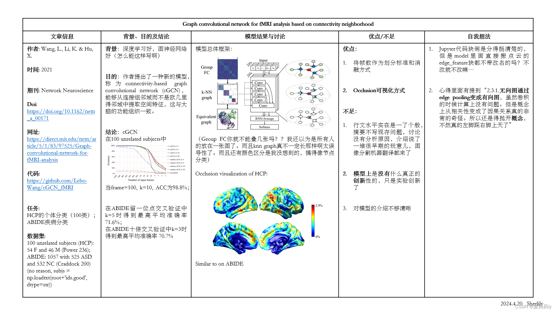
 本文介绍了一种名为cGCN的图卷积网络,用于fMRI数据分析,特别关注基于邻接性的方法。论文探讨了深度学习在fMRI数据和FC矩阵上的应用,以及cGCN的构建、边缘函数和实验设置。研究发现cGCN性能受邻居数量和输入帧数影响,并通过occlusionmethod进行了可视化分析。作者讨论了模型选择和可视化挑战,指出边缘kNN方法的优点。
英文是纯手打的!论文原文的summarizing and paraphrasing。可能会出现难以避免的拼写错误和语法错误,若有发现欢迎评论指正!文章偏向于笔记,谨慎食用
目录
2.2.1. Deep Learning on fMRI Data
2.2.2. Deep Learning on FC Matrix
2.2.3. Graph Convolutional Networks
2.3.3. The Edge Function of cGCN
2.3.4. Experiments and Settings
2.4.1. Performance Related to the Number of Neighbors
2.4.2. Performance Related to the Number of Input Frames
1. 省流版
1.1. 心得
(1)模型介绍好少,我也不知道创新到哪了...可能没人这样缝
(2)好像没咋见过这种按帧数来消融的
(3)不能来个精度表是吧
(4)⭐比较独特的occlusion method可视化
(5)⭐⭐2.3.1.无向图通过edge pooling变成有向图,虽然卷积的时候计算上没有问题。但是概念上从相关性变成了因果关系真的非常的奇怪。所以还是得抛开概念,不然真的左脚踩右脚上天了
(6)论作者如何从1112个数据中选出1057个:subjs = np.loadtxt(root+'ids.good', dtype=str)。好像在和我开玩笑一样
1.2. 论文总结图
2. 论文逐段精读
2.1. Abstract
①They proposed a connectivity-based graph convolutional network (cGCN)
2.2. Introduction
①Methods of FC analyses: sliding-window, time-frequency, and the Gaussian hidden Markov model
2.2.1. Deep Learning on fMRI Data
①Introducing several CNN models applied to neuroimaging field
②⭐Limitation of CNN on brain analysis:
| (a) | computation costs |
| (b) | unnecessary white matter convolution |
| (c) | noise in time series signals of single voxel |
| (d) | can not aggregate node information from distant nondes |
2.2.2. Deep Learning on FC Matrix
①Introducing deep learning on FC
2.2.3. Graph Convolutional Networks
①GCN contains spectral GCNs and spatial GCNs
2.3. Materials and Methods
2.3.1. cGCN Overview
①Overall framework of cGCN:
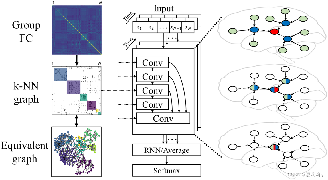
这个图的kNN有点问题,在作者给出的代码中的random-FC的kNN长这样:
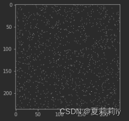
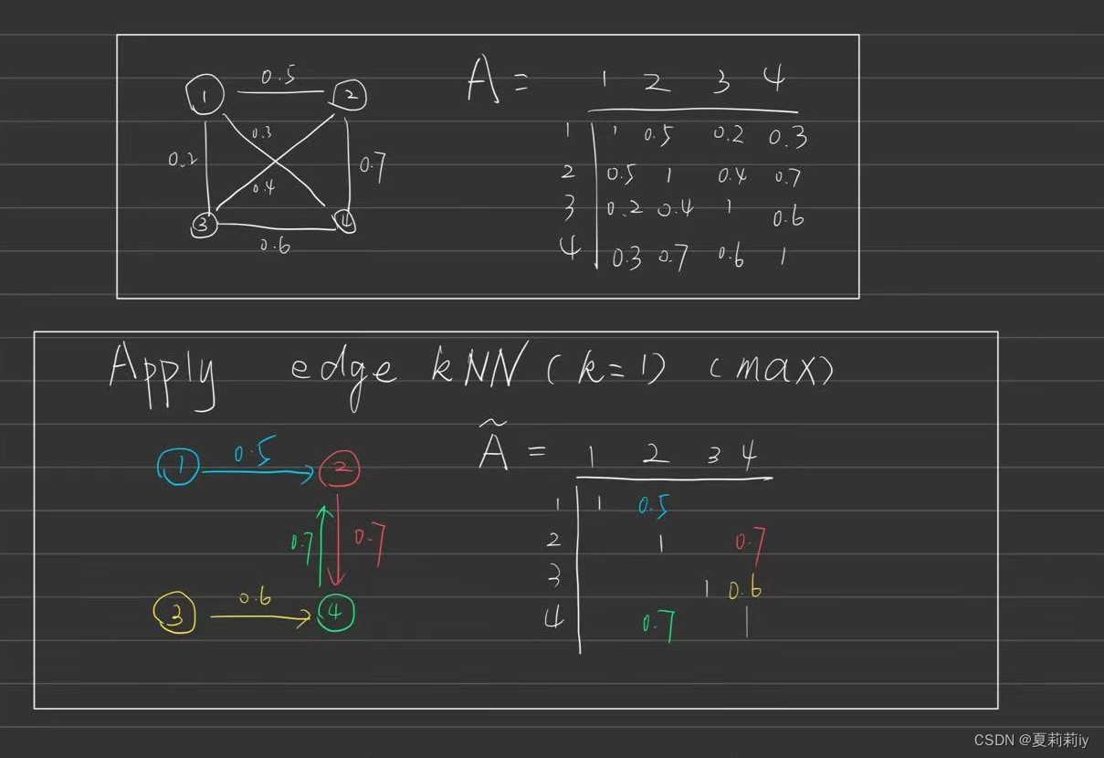
它其实不太是上面那种都聚合在中间的正方形。其次,⭐它从有向图变成了无向图。
原因和示例如下:
其次,代码中用ConvLSTM2D代替了RNN
②Only leaving the top-k edges of one node (k=3, 5, 10, 20)
2.3.2. Graph Construction
①Channel: each frame of fMRI data
2.3.3. The Edge Function of cGCN
①Convolutional method: EdgeConv (GCN)
where denotes non-linear activation function with trainable weight
(这x都是节点特征啊,这文章没有边缘特征和边缘权重=,=,代码叫Edge_feature...有点恶心了不是?
![]()
我以为真Edge feature,但是查了PyG的EdgeConv是酱紫的:
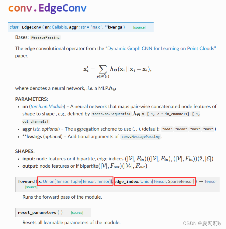
输入压根就没有Edge_feature捏,所以只是knn给每个节点留个k个边,再从这剩下的边里面找节点特征最大的neighbor)
2.3.4. Experiments and Settings
(1)HCP
①Dataset: 100 unrelated subjects
②Sample: 100 with 54 females and 46 males
③Preprocessing: HCP minimal preprocessing pipeline
④Atlas: Power 236
⑤Training set: two sessions from Day 1 with 100 frames per channel
⑥Validation set: two sessions from Day 2 from 1 to 1200 frames(截取的1200,600,400一直往下,这样)
⑦⭐Task: individual identification, 100 classifications (each subject gets 4 sessions of fMRI scanning with 1200 volumn per session)
(2)ABIDE
①Sample: 1057 with 525 ASD and 532 NC
②Preprocessing: Connectome Computation System pipeline
③Atlas: Craddock 200
④Validation: leave-one-site-out and tenfold cross-validation
(3)Settings
①Optimizer: Adam
②Weight decay: stepwise when there is no fluctuation
③Minimum learning rate: 1e-6
④Regularization: L2 (0.1, 0.01, 0.001, and 0.0001)
2.3.5. Visualization
①Important ROIs visualization: occlusion method
②Steps: masking each ROI to measure the performance decrease
2.4. Results
2.4.1. Performance Related to the Number of Neighbors
①Ablation study of k on HCP:
it achieves the highest performance when k=5(当input frame=1的时候是哪一帧?)
②Leave-one-site-out and 10 fold cross-validation on ABIDE:
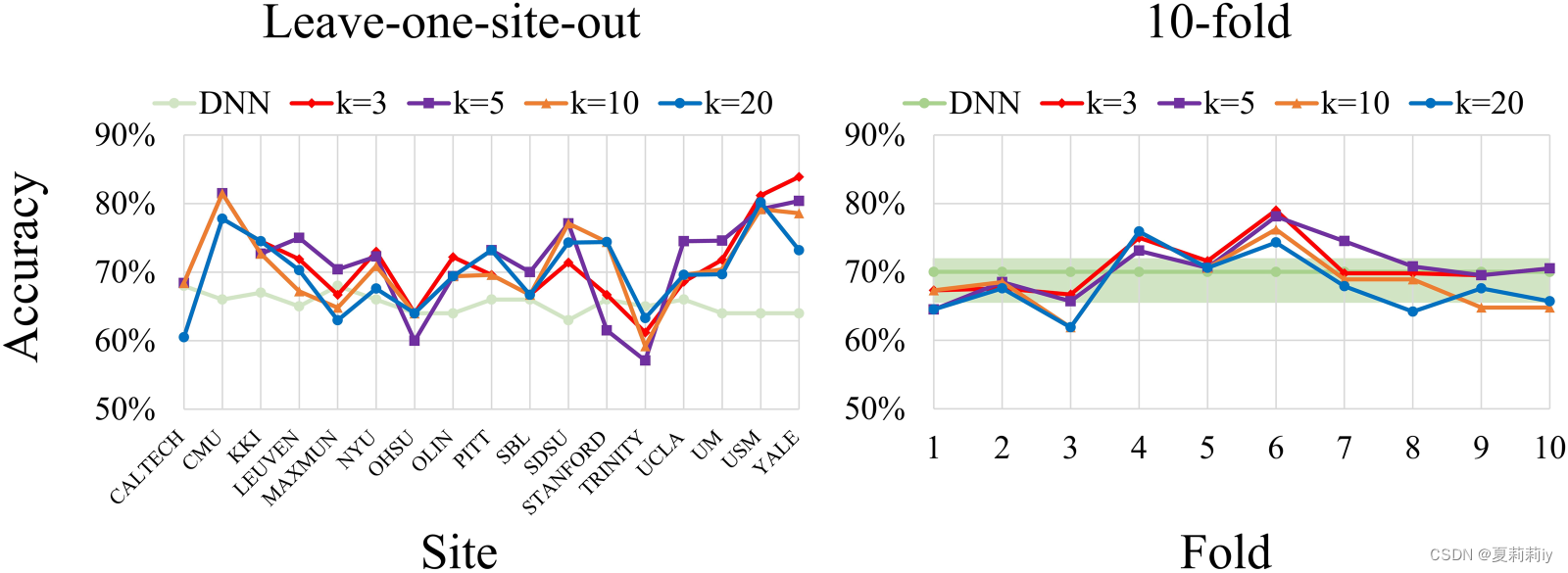
the best average performance on leave-one-site-out is 71.6% when k=5 and on 10 fold is 70.7% when k=3
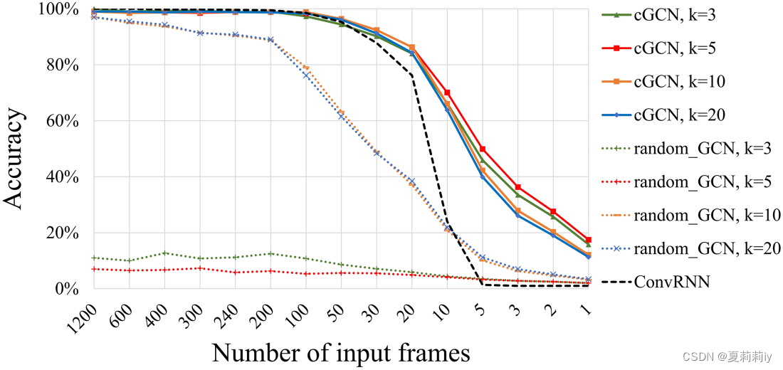
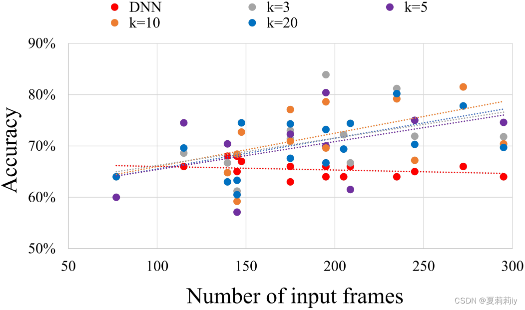
2.4.2. Performance Related to the Number of Input Frames
①How frames influence ASD classification:
2.4.3. Comparison
①The best performance: 98.8% when k=10 and frames=100 on HCP
2.4.4. Visualization
①For HCP, the minimum accuracy decrease is 0.6% when k=20 and the maximum one is 2.9% when k=3
②Visualization on HCP:
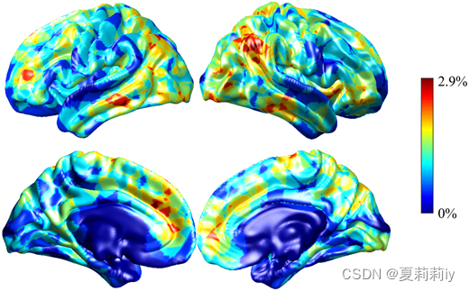
where default mode network, frontoparietal network, and visual network contribute to individual classification
③The average performance degradation on leave-one-site-out cross-validation on ABIDE:
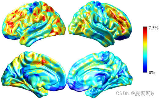
the minimum accuracy decrease is 6% when k=20 and the maximum one is 7.5% when k=20. Moreover, the salient regions of ASD classification are frontoparietal network, default mode network, and ventral attention network.
2.5. Discussion
①⭐作者认为边缘knn比硬阈值好因为每个点边缘数量相同适用于卷积(需要你来适用吗??什么理由啊)
②⭐It is hard to visualize temporal information connectomic neighborhoods
2.6. Conclusion
cGCN caputures node information from
3. 知识补充
3.1. Occlusion method
(1)定义:
深度学习的Occlusion method(遮挡法)是一种常用的扰动法,用于评估输入数据不同部分对模型输出的影响。这种方法的基本思想是通过遮挡输入数据的一部分(例如,将输入像素的一部分置为零或将其特征值设为零),然后观察模型输出的变化。如果输出变化较大,则说明被遮挡的部分对模型预测结果的重要性较高。
遮挡法在许多机器学习模型上都有所应用,特别是在处理图像和文本数据时。对于图像数据,遮挡法可以通过将图像的一部分像素置为零来遮挡特定的区域;对于文本数据,遮挡法则可以通过将某个单词或词组的嵌入向量置为零来实现遮挡。
遮挡法的优势在于其实现简单且不需要反向传播,因此运行速度相对较快。然而,需要注意的是,遮挡法只能提供关于被遮挡部分重要性的局部信息,而不能全面反映整个输入数据对模型输出的影响。
(2)参考论文:1311.2901.pdf (arxiv.org)
4. Reference List
Wang, L., Li, K. & Hu, X. (2021) 'Graph convolutional network for fMRI analysis based on connectivity neighborhood', Network Neuroscience, 5 (1), pp. 83-95. doi: Graph convolutional network for fMRI analysis based on connectivity neighborhood | Network Neuroscience | MIT Press


 1万+
1万+

 被折叠的 条评论
为什么被折叠?
被折叠的 条评论
为什么被折叠?
 到【灌水乐园】发言


