


Llama3复现
0 前言
Llama 3,是Meta公司发布的大型语言模型,虽然能力上不如GPT4,但因为GPT4不开源,所以截至2024年4月,它也是最强的开源大模型。Llama3 有 8B 和 70B 两个版本。无论哪一个,我们都不可能成功复现出来,所以今天我们只实现一个mini版本,即原模型有的结构这里都有,但层数和维度都做了简化,其中隐藏层维度由4096降为1024,解码层数量由32降为2。
本文的内容参考了B站up主蓝斯诺特的视频和代码。
1 注意力机制与位置编码
1.1 注意力机制
Llama3是Decoder-Only结构,它和 GPT2 最明显的区别就是注意力机制这一块。Llama3中,将位置编码融入到了注意力机制当中,它的代码主体结构如下:
import torch
import math

#注意力层
class LlamaAttention(torch.nn.Module):

    def __init__(self, d_k):
        super().__init__()
        self.q_proj = torch.nn.Linear(1024, 1024, bias=False)

        # 注意,这里KV被降维了,而transformer中却没有
        self.k_proj = torch.nn.Linear(1024, 256, bias=False)
        self.v_proj = torch.nn.Linear(1024, 256, bias=False)

        self.o_proj = torch.nn.Linear(1024, 1024, bias=False)

        self.d_k = d_k

    def forward(self, hidden_states, attention_mask):
        """

        Args:
            hidden_states: [4, 125, 1024]
            attention_mask: [4, 125]

        Returns:

        """
        b, lens, d_model = hidden_states.shape
        h_q = d_model // self.d_k  # 32 = 1024 // 32
        h_kv = int(h_q / 4)

        assert d_model % self.d_k == 0
        assert  h_kv % 4 == 0

        # 线性投影获得qkv,并拆分成多头
        # [4, 125, 1024] -> [4, 125, 1024] -> [4, 125, 32, 32] -> [4, 32, 125, 32]
        q = self.q_proj(hidden_states).reshape(b, lens, h_q, self.d_k).transpose(1, 2)
        # [4, 125, 1024] -> [4, 125, 256] -> [4, 125, 8, 32] -> [4, 8, 125, 32]
        k = self.k_proj(hidden_states).reshape(b, lens, h_kv, self.d_k).transpose(1, 2)
        # [4, 125, 1024] -> [4, 125, 256] -> [4, 125, 8, 32] -> [4, 8, 125, 32]
        v = self.v_proj(hidden_states).reshape(b, lens, h_kv, self.d_k).transpose(1, 2)

        # 计算位置编码
        # [1, 125, 32],[1, 125, 32]
        cos, sin = llama_rotary_embedding(lens, self.d_k)
        cos, sin = cos.to(hidden_states.device), sin.to(hidden_states.device)

        # 在q,k上应用位置编码
        # [4, 32, 125, 32] -> [4, 32, 125, 32]
        q = apply_rotary_pos_emb(q, cos, sin)
        # [4, 8, 125, 32] -> [4, 8, 125, 32]
        k = apply_rotary_pos_emb(k, cos, sin)

        # kv 复制4分,方便后面与 q 进行矩阵运算
        # [4, 8, 125, 32] -> [4, 32, 125, 32]
        k = repeat_kv(k)
        # [4, 8, 125, 32] -> [4, 32, 125, 32]
        v = repeat_kv(v)

        # 计算注意力得分
        # [4, 32, 125, 32] * [4, 32, 32, 125] -> [4, 32, 125, 125]
        scores = q.matmul(k.transpose(2, 3)) / math.sqrt(32)

        # 根据attention_mask获得注意力遮罩
        # [4, 125] -> [4, 1, 125, 125]
        attention_mask = get_causal_mask(attention_mask)

        # 计算注意力权重
        # [4, 32, 125, 125] + [4, 1, 125, 125] -> [4, 32, 125, 125]
        p_attn = (scores + attention_mask).softmax(3)

        # 对v中的向量进行加权
        # [4, 32, 125, 125] * [4, 32, 125, 32] -> [4, 32, 125, 32]
        attn = p_attn.matmul(v)

        # 合并多头注意力
        # [4, 32, 125, 32] -> [4, 125, 32, 32] -> [4, 125, 1024]
        attn = attn.transpose(1, 2).reshape(b, lens, 1024)

        # 线性输出
        # [4, 125, 1024] -> [4, 125, 1024]
        attn = self.o_proj(attn)

        return attn
熟悉 Transformer 的同学,对 forward 函数的过程不难看懂,这里调用了几个函数:llama_rotary_embedding、apply_rotary_pos_emb、repeat_kv、get_causal_mask,我们来逐个讲解。
先说一下最简单的repeat_kv,它其实就是扩展KV,使其和Q的维度相同:
def repeat_kv(x):
    shape = list(x.shape)
    shape[1] *= 4
    #[4, 8, 125, 32] -> [4, 8, 1, 125, 32] -> [4, 8, 4, 125, 32] -> [4, 32, 125, 32]
    return x.unsqueeze(2).repeat(1, 1, 4, 1, 1).reshape(shape)
接下来是获取遮罩矩阵,它就是获取一个上三角矩阵(不含对角线),对角线及对角线以下部分都为0,对角线以上部分为负无穷大,与此同时,遮罩中对应原句子为填充部分的,也要将其转为无穷小。下面的代码看不懂也没关系。只需要知道它的输入输出是怎么样的就OK:
# 根据attention_mask获取注意力遮罩
# 遮罩值为0表示保留,min_value表示丢弃
# 遮罩的用法是和注意力得分(对齐分数)矩阵相加后再求softmax
def get_causal_mask(attention_mask):
    # attention_mask -> [4, 125]

    b, lens = attention_mask.shape
    min_value = -1e15	# 这个数可以认为是负无穷大了

    #上三角矩阵,对角线以上为min_value,对角线以下为0,对角线为0
    #[4, 1, 125, 125]
    causal_mask = torch.full((lens, lens), min_value).triu(diagonal=1)
    causal_mask = causal_mask.reshape(1, 1, lens, lens).repeat(b, 1, 1, 1)
    causal_mask = causal_mask.to(attention_mask.device)

    # 是pad的位置填充为min_value
    # [4, 125] -> [4, 1, 1, 125]
    mask = attention_mask.reshape(b, 1, 1, lens) == 0
    # [4, 1, 125, 125]
    causal_mask = causal_mask.masked_fill(mask, min_value)

    return causal_mask
可以测试以下:
if __name__ == '__main__':
    att_mask = get_causal_mask(torch.ones(1, 5).long())
    print(att_mask)
输出:
tensor([[[[ 0.0000e+00, -1.0000e+15, -1.0000e+15, -1.0000e+15, -1.0000e+15],
          [ 0.0000e+00,  0.0000e+00, -1.0000e+15, -1.0000e+15, -1.0000e+15],
          [ 0.0000e+00,  0.0000e+00,  0.0000e+00, -1.0000e+15, -1.0000e+15],
          [ 0.0000e+00,  0.0000e+00,  0.0000e+00,  0.0000e+00, -1.0000e+15],
          [ 0.0000e+00,  0.0000e+00,  0.0000e+00,  0.0000e+00,  0.0000e+00]]]])
1.2 位置编码
接下来我们说一下位置编码,Llama3中用的是旋转位置编码(Rotary Positional Embedding, RoPE)。
我们先说一下基本的位置编码,公式如下:
P
E
c
o
s
(
p
o
s
,
2
i
)
=
c
o
s
(
p
o
s
50000
0
2
i
/
d
k
)
P
E
s
i
n
(
p
o
s
,
2
i
)
=
s
i
n
(
p
o
s
50000
0
2
i
/
d
k
)
\begin{aligned} PE_{cos}(pos, 2i) = cos(\frac{pos}{500000^{2i/d_k}})\\ PE_{sin}(pos, 2i) = sin(\frac{pos}{500000^{2i/d_k}}) \end{aligned}
PEcos(pos,2i)=cos(5000002i/dkpos)PEsin(pos,2i)=sin(5000002i/dkpos)
代码如下:
# 计算结果是常量,有必要的话可以保存起来节省计算资源
@torch.no_grad()
def llama_rotary_embedding(lens, d_k):
	"lens是句子长度, d_k是每个注意力头的编码维度"
    # 生成维度索引
    d_i = torch.arange(0, d_k, 2) / d_k     # [d_k/2]

    # 角速度 w
    omega = 1.0 / (50_0000.0 ** d_i)
    omega = omega.reshape(1, 16, 1)  # [d_k/2] -> [1, d_k/2, 1]

    # 生成位置索引,[1, 1, lens]
    position_ids = torch.arange(lens).reshape(1, 1, -1).float()

    # 位置索引与频率维度相乘,构建cos(wx)与sin(wx)中的 wx
    # [1, d_k/2, 1] matmul [1, 1, lens] -> [1, d_k/2, lens] -> [1, lens, d_k/2]
    freqs = omega.matmul(position_ids).transpose(1, 2)

    # freqs复制一份,一份用于偶数位置(cos),另一份用于奇数(sin)
    emb = torch.cat((freqs, freqs), 2)  # [1, lens, d_k]

    return emb.cos(), emb.sin()
上述代码是获得两个矩阵,分别是余弦与正弦。接下来要将这两个矩阵用到q和k上面,这里涉及到了一个名为apply_rotary_pos_emb的函数,它的过程如下:
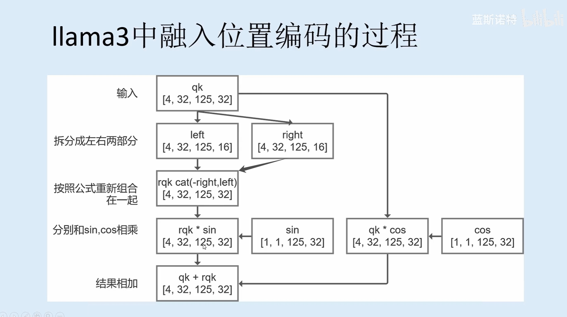
其代码如下:
def apply_rotary_pos_emb(x, cos, sin):
    """
    应用旋转位置嵌入到输入张量x上。

    参数:
    x (torch.Tensor): 输入张量,形状为[batch_size, n_heads, lens, d_k]。
    cos (torch.Tensor): 余弦部分的位置嵌入,形状为[1, lens, d_k]。
    sin (torch.Tensor): 正弦部分的位置嵌入,形状为[1, lens, d_k]。

    返回:
    torch.Tensor: 应用了旋转位置嵌入后的输出张量,形状与输入张量x相同。
    """

    def rotate_half(x, d_k):
        """
        将输入张量的最后一个维度分成两半,并进行旋转操作。

        参数:
        x (torch.Tensor): 输入张量 [batch_size, n_heads, lens, d_k]
        d_k (torch.Tensor): 每个注意力头的维度

        返回:
        torch.Tensor: 旋转后的输出张量。
        """

        # 将输入张量的最后一个维度分成两半
        left = x[..., :d_k//2]
        right = x[..., d_k//2:]

        # 将右半部分的相反数放在左半部分前面,实现旋转效果
        # [batch_size, n_heads, lens, d_k] -> [batch_size, n_heads, lens, d_k] -> [batch_size, n_heads, lens, d_k]
        return torch.cat((-right, left), -1)

    # [1, lens, d_k] -> [1, 1, lens, d_k]
    cos = cos.unsqueeze(1)
    # [1, lens, d_k] -> [1, 1, lens, d_k]
    sin = sin.unsqueeze(1)

	d_k = x.shape[-1]
    # 将输入张量x与扩展后的余弦位置嵌入相乘,再加上旋转一半后的x与扩展后的正弦位置嵌入的乘积
    x = (x * cos) + (rotate_half(x, d_k) * sin)		# [batch_size, n_heads, lens, d_k]

    # 返回应用了旋转位置嵌入后的输出张量
    return x
这个过程是比较难理解的,这里理解不了也不要紧,可以看这个视频和这篇文章
文章中的公式是这样的:
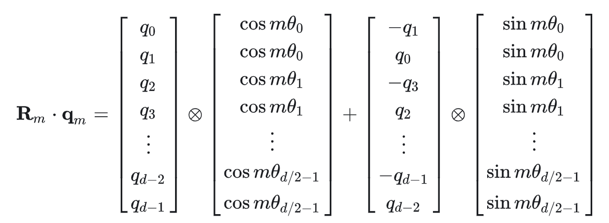
和我们的代码不能完全对应起来,但没关系,因为这只是空间中的排列顺序的区别,每个子空间中的维度是独立的,只需要把注意力头的编码维度两两分组就行,是相邻两个维度一组,还是说把前后相隔d_k/2的两个维度分为一组,其实从空间的角度来看没差。
1.3 注意力机制测试代码
if __name__ == '__main__':
    input = {
        'hidden_states': torch.randn(4, 125, 1024),
        'attention_mask': torch.ones(4, 125)
    }
    print(LlamaAttention(d_k=32)(**input).shape)
输出
torch.Size([4, 125, 1024])
2 归一化层与FFN
2.1 RMS Norm 层
Llama3的归一化层延续了Llama系列前几代的设计,采用了RMS Normalization(Root Mean Square Normalization),简称均方根归一化。以下是关键细节:
-
1 公式:对于输入向量 x,归一化公式为:
RMSNorm ( x ) = x mean ( x 2 ) + ϵ ⋅ γ \operatorname{RMSNorm}(x)=\frac{x}{\sqrt{\operatorname{mean}\left(x^{2}\right)+\epsilon}} \cdot \gamma RMSNorm(x)=mean(x2)+ϵx⋅γ
其中, γ \gamma γ 是可学习的缩放参数, ϵ \epsilon ϵ 是为数值稳定性添加的小常数(如 1e−6)。 -
2 相比于层归一化,RMS Norm仅基于输入特征的均方根值(RMS)进行缩放,省去了均值中心化的步骤,从而减少计算量(省略均值计算,降低约10%的计算开销)。
-
3 位置与结构:Pre-LN 结构:归一化层位于每个Transformer子层(自注意力、前馈网络)之前(Pre-Layer Normalization),而非之后。这种设计提升了训练稳定性,尤其在深层网络中。
-
4 残差连接:每个子层的输出通过 x+Sublayer(Norm(x)) 实现,即归一化后的结果经子层处理,再与原始输入相加。
优势:
训练稳定性:Pre-LN + RMS Norm + 残差连接的组合有效缓解了梯度消失/爆炸问题,适合大规模模型训练。
代码:
# Norm层
class LlamaRMSNorm(torch.nn.Module):

    def __init__(self):
        super().__init__()
        self.weight = torch.nn.Parameter(torch.ones(1024))

    def forward(self, x):
        #[4, 125, 1024] -> [4, 125, 1]
        var = x.pow(2).mean(2, keepdim=True)

        # 差不多相当于x除以自身的绝对值的均值,相当于一种缩放
        # 计算结果的均值总是在-1到1之间
        # [4, 125, 1024] * [4, 125, 1] -> [4, 125, 1024]
        x = x * (var + 1e-5).rsqrt()	# .rsqrt()的作用是开方后取倒数

        # [1024] * [4, 125, 1024] -> [4, 125, 1024]
        return self.weight * x

if __name__ == '__main__':
	print(LlamaRMSNorm()(torch.randn(4, 125, 1024)).shape)
输出:
torch.Size([4, 125, 1024])
2.2 FFN结构
Llama3 的FFN层有以下细节:
-
1 门控结构:采用 SwiGLU 激活函数(Sigmoid-Weighted Linear Unit),包含两个并行的线性层,通过门控机制增强非线性表达能力,再通过第三个线性层恢复原始维度,适配残差连接。
-
2 SwiGLU 激活函数(Sigmoid-Weighted Linear Unit):
- 表达式为 SwiGLU ( x ) = swish ( x W 1 ) ⊗ x W 2 \operatorname{SwiGLU}(x)=\operatorname{swish}\left(x W_{1}\right) \otimes x W_{2} SwiGLU(x)=swish(xW1)⊗xW2,其中 swish 激活函数的表达式为 x ⋅ s i g m o i d ( β x ) x \cdot sigmoid(\beta x) x⋅sigmoid(βx)
- SwiGLU是带可训练参数的激活函数,整个FFN结构可以看成 SwiGLU+线性层;
- 与ReLU相比,由于 swish 的存在,SwiGLU具有平滑性,与GELU相比,SwiGLU计算复杂度较小,综合来看,SwiGLU梯度稳定性最优
-
3 线性层不包含偏置参数(bias=False),这是因为:
- 归一化层的作用:前置的 RMS 归一化已对输入分布进行中心化处理,偏置的调整作用被冗余化;
- 减少参数量:对于超大规模模型(如千亿参数),去除偏置可显著降低显存占用和计算开销。
代码如下:
class LlamaFFN(torch.nn.Module):

    def __init__(self):
        super().__init__()
        # 门控线性层
        self.gate_proj = torch.nn.Linear(1024, 14336, bias=False)
        self.up_proj = torch.nn.Linear(1024, 14336, bias=False)
        # 输出投影层
        self.down_proj = torch.nn.Linear(14336, 1024, bias=False)
        # silu激活函数(silu等价于swish(beta=1))
        self.act_fn = torch.nn.SiLU()

    def forward(self, x):
        #[4, 125, 1024] -> [4, 125, 14336]
        left = self.act_fn(self.gate_proj(x))

        #[4, 125, 1024] -> [4, 125, 14336]
        right = self.up_proj(x)

        #[4, 125, 14336] -> [4, 125, 1024]
        return self.down_proj(left * right)


if __name__ == '__main__':
    print(LlamaFFN()(torch.randn(4, 125, 1024)).shape)
输出
torch.Size([4, 125, 1024])
3 Llama3 的解码层
介绍完 Llama3 的所有组件后,我们可以来搭建解码层了:
class LlamaDecoderLayer(torch.nn.Module):

    def __init__(self, d_k):
        super().__init__()
        self.self_attn = LlamaAttention(d_k)
        self.ffn = LlamaFFN()
        self.input_layernorm = LlamaRMSNorm()
        self.post_attention_layernorm = LlamaRMSNorm()

    def forward(self, hidden_states, attention_mask):
        # hidden_states -> [batch_size, lens, d_model]
        # attention_mask -> [batch_size, lens]

        res = hidden_states

        # norm
        # [batch_size, lens, d_model] -> [batch_size, lens, d_model]
        hidden_states = self.input_layernorm(hidden_states)

        # 计算注意力,短接
        # [batch_size, lens, d_model], [batch_size, lens] + [batch_size, lens, d_model] -> [batch_size, lens, d_model]
        hidden_states = self.self_attn(hidden_states=hidden_states,
                                       attention_mask=attention_mask) + res
        res = hidden_states

        # norm
        # [batch_size, lens, d_model] -> [batch_size, lens, d_model]
        hidden_states = self.post_attention_layernorm(hidden_states)

        # 线性计算,短接
        # [batch_size, lens, d_model] + [batch_size, lens, d_model] -> [batch_size, lens, d_model]
        hidden_states = self.ffn(hidden_states) + res

        return hidden_states

if __name__ == '__main__':
    input = {
        'hidden_states': torch.randn(4, 125, 1024),
        'attention_mask': torch.ones(4, 125).long()
    }
    print(LlamaDecoderLayer(d_k=32)(**input).shape)
输出:
torch.Size([4, 125, 1024])
4 Llama3的完整结构
class LlamaModel(torch.nn.Module):
    """
    Llama模型的主要结构。

    参数:
    - d_model: 模型的维度。
    - d_k: 注意力头的维度。
    - num_decoder: 解码器层的数量。

    注意:通过初始化时的断言确保d_model可以被d_k整除。
    """

    def __init__(self, d_model, d_k, num_decoder):
        super().__init__()
        # 确保d_model可以被d_k整除,这对于多头注意力机制是必要的。
        assert d_model % d_k == 0

        # 词汇嵌入层,将输入的token ID转换为模型维度的向量。
        self.embed_tokens = torch.nn.Embedding(128256, d_model, None)

        # 使用ModuleList创建解码器层的列表,每个元素都是一个LlamaDecoderLayer实例。
        self.layers = torch.nn.ModuleList(
            [LlamaDecoderLayer(d_k) for _ in range(num_decoder)])

        # 最后的归一化层,用于对隐藏状态进行归一化。
        self.norm = LlamaRMSNorm()

    def forward(self, input_ids, attention_mask):
        """
        参数:
        - input_ids: 输入的token ID序列,形状为[batch_size, sequence_length]。
        - attention_mask: 注意力掩码,用于指示每个位置是否应该被关注。

        返回:
        - hidden_states: 最终的隐藏状态序列。
        """
        # input_ids -> [batch_size, sequence_length]
        # attention_mask -> [batch_size, sequence_length]

        # 编码
        # [batch_size, sequence_length] -> [batch_size, sequence_length, d_model]
        hidden_states = self.embed_tokens(input_ids)

        # n层计算
        for layer in self.layers:
            # [batch_size, sequence_length, d_model] -> [batch_size, sequence_length, d_model]
            hidden_states = layer(hidden_states, attention_mask=attention_mask)

        # norm
        # [batch_size, sequence_length, d_model] -> [batch_size, sequence_length, d_model]
        hidden_states = self.norm(hidden_states)

        return hidden_states


if __name__ == '__main__':
    input = {
        'input_ids': torch.randint(100, 50000, [4, 125]),
        'attention_mask': torch.ones(4, 125).long(),
    }
    input['attention_mask'][:, 120:] = 0
    print(LlamaModel(1024, 32, 2)(**input).shape)
接下来是因果模型(即能把模型的输出转成softmaxt之前的逻辑值,以及计算损失函数):
class LlamaForCausalLM(torch.nn.Module):
    def __init__(self):
        super().__init__()
        self.model = LlamaModel(1024, 32, 2)
        self.lm_head = torch.nn.Linear(1024, 128256, bias=False)

    def forward(self, input_ids, attention_mask, labels=None):
        # input_ids -> [batch_size, lens]
        # attention_mask -> [batch_size, lens]
        # labels -> [batch_size, lens]

        # [batch_size, lens] -> [batch_size, lens, d_model]
        logits = self.model(input_ids=input_ids, attention_mask=attention_mask)

        # [batch_size, lens, d_model] -> [batch_size, lens, vocab_size]
        logits = self.lm_head(logits)

        loss = None
        if labels is not None:
            shift_logits = logits[:, :-1].reshape(-1, 128256)
            shift_labels = labels[:, 1:].reshape(-1)
            loss = torch.nn.functional.cross_entropy(shift_logits,
                                                     shift_labels)

        return loss, logits


if __name__ == '__main__':
    input = {
        'input_ids': torch.randint(100, 50000, [4, 125]),
        'attention_mask': torch.ones(4, 125).long(),
        'labels': torch.randint(100, 50000, [4, 125]),
    }
    input['attention_mask'][:, 120:] = 0
    loss, logits = LlamaForCausalLM()(**input)
    print(loss, logits.shape)
输出:
tensor(11.9515, grad_fn=<NllLossBackward0>) torch.Size([4, 125, 128256])
5 总结
相比于Transformer与GPT2,Llama3的特点包括以下几点:
- 1 在注意力机制内部插入位置编码;
- 2 位置编码使用旋转位置编码;
- 3 归一化层使用 RMS Norm,在注意力模块前面和后面均有归一化层;
- 4 FFN 结构采用 SwiGLU 激活函数。
面试的时候,能答出以上几点,基本上就不会有什么大问题。


 20万+
20万+

 被折叠的 条评论
为什么被折叠?
被折叠的 条评论
为什么被折叠?
 到【灌水乐园】发言


