PCoA+boxplot：宏基因组扩增子组间差异分析（Beta多样性组合图）

 数据和代码获取：请查看主页个人信息！！！

大家好，今天我将介绍如何使用R语microeco包进行beta多样性分析，并进行PCoA+boxplot组合图展示。

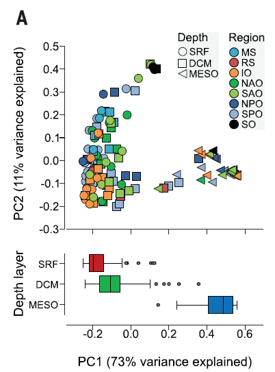
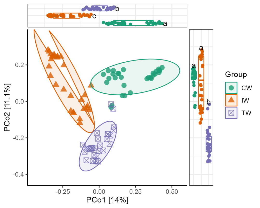
这种组合图的优势在于不仅可以展示样本的群落组成差异，可以展示不同分组样本在主成分上的分离情况：

接下来我们来进行分析和可视化展示：

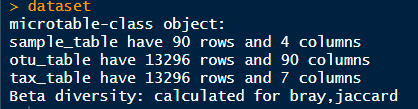
Step1：创建microtable对象

rm(list=ls())pacman::p_load(tidyverse,microeco,aplot,ggsci)
feature_table <- read.csv('feature_table.csv', row.names = 1)sample_table <- read.csv('sample_table.csv', row.names = 1)tax_table <- read.csv('tax_table.csv', row.names = 1)
# 创建microtable对象dataset <- microtable$new(sample_table = sample_table,                          otu_table = feature_table,                           tax_table = tax_table)dataset

Step2：执行PCoA分析

# PCoAdataset$cal_betadiv()t1 <- trans_beta$new(dataset = dataset, group = "Group", measure = "bray")t1$cal_ordination(ordination = "PCoA")tmp <- t1$res_ordination$scores# differential test with trans_env classt2 <- trans_env$new(dataset = dataset, add_data = tmp[, 1:2])# 'KW_dunn' for non-parametric testt2$cal_diff(group = "Group", method = "anova")t2

这里我们首先计算了beta距离，然后执行了PCoA分析；同时进行差异检验。

Step3：使用t1和t2对象中的绘图函数进行可视化

# 然后，使用t1和t2对象中的绘图函数进行可视化。p1 <- t1$plot_ordination(plot_color = "Group", plot_shape = "Group", plot_type = c("point", "ellipse"))
p2 <-   t2$plot_diff(measure = "PCo1", add_sig = T) +   theme_bw() +   coord_flip() +   theme(legend.position = "none",         axis.title.x = element_blank(),         axis.text.y = element_blank(),         axis.ticks.y = element_blank())
p3 <- t2$plot_diff(measure = "PCo2", add_sig = T) +   theme_bw() +   theme(legend.position = "none",         axis.title.y = element_blank(),         axis.text.x = element_blank(),         axis.ticks.x = element_blank())
g <- p1 %>%   insert_top(p2, height = 0.2) %>%   insert_right(p3, width = 0.2)g

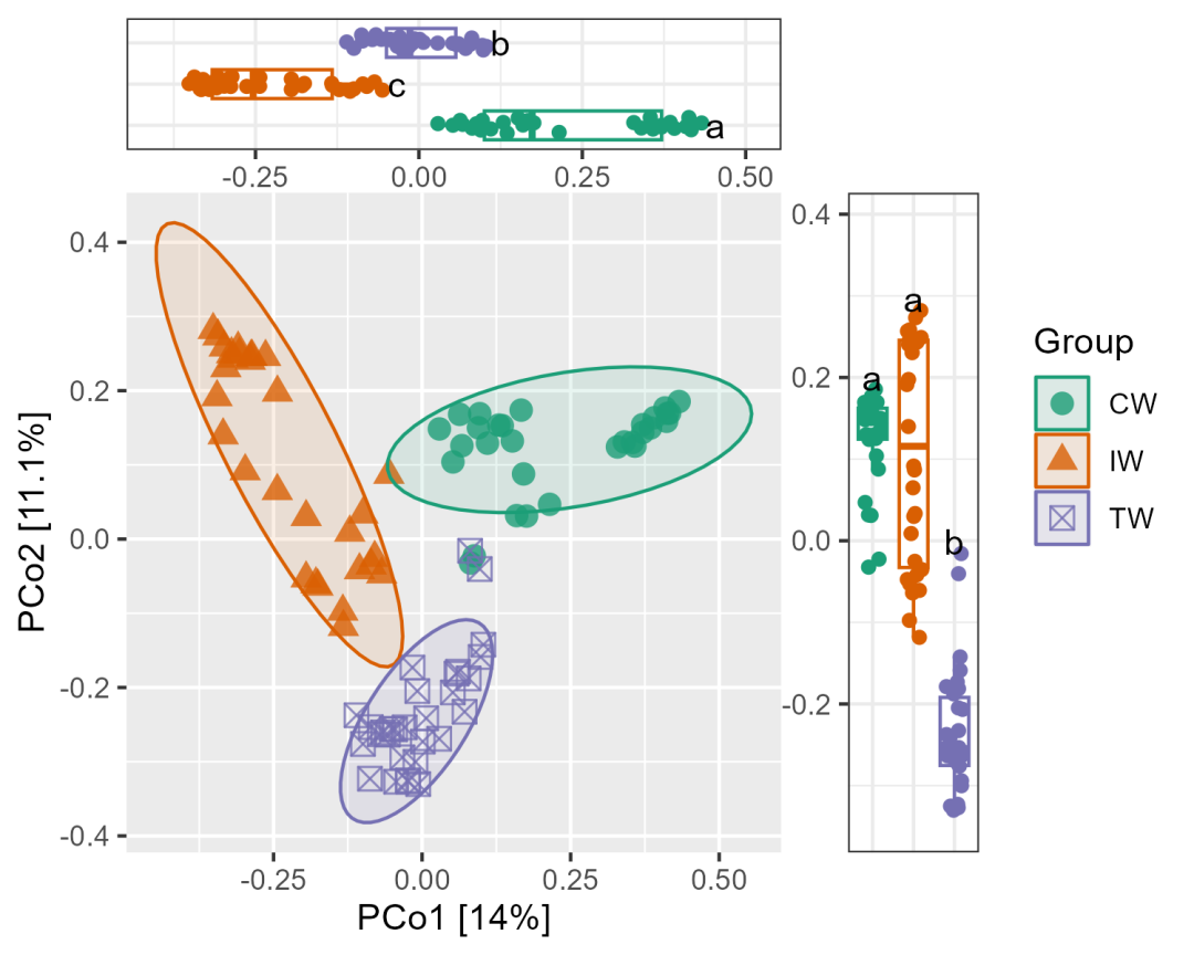
在这一点上，我们注意到上图的水平轴和右侧图的垂直轴与主图的轴线并不完全对应。因此，如果我们继续使用这些图形，应该保留上图和右侧图的刻度线。如果用户需要完全对应的刻度线，则需要进一步控制坐标轴。

我们手动控制坐标范围：

Step4：手动控制坐标范围

x_lim <- range(tmp[, 1]) * 1.4y_lim <- range(tmp[, 2]) * 1.4
p1 <- p1 + scale_y_continuous(limits = y_lim, expand = c(0, 0)) +   scale_x_continuous(limits = x_lim, expand = c(0, 0))
p2 <- p2 + scale_y_continuous(limits = x_lim, expand = c(0, 0))
p3 <- p3 + scale_y_continuous(limits = y_lim, expand = c(0, 0))
g <- p1 %>%   insert_top(p2, height = 0.2) %>%   insert_right(p3, width = 0.2)g

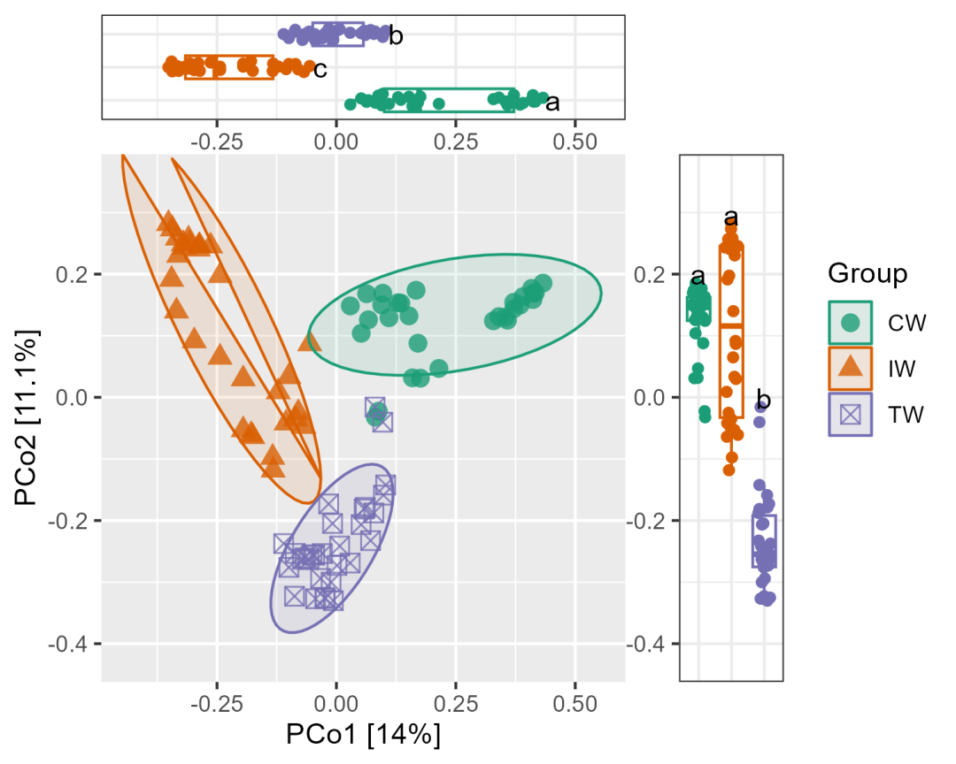
Step5：对齐刻度线

p2 <- p2 + theme(axis.text.x = element_blank(), axis.ticks.x = element_blank())p3 <- p3 + theme(axis.text.y = element_blank(), axis.ticks.y = element_blank())g <- (p1 + theme_classic()) %>%   insert_top(p2, height = 0.15) %>%   insert_right(p3, width = 0.15)g

本期分享到此结束~~~本期内容主要通过microeco包实现分析和可视化，我个人推荐大家用这个包来进行微生物常见的分析，真的会节约大量时间。

当然，本期的分析内容也可以通过vegan包分析+ggplot2包实现，有必要的话我会单独写一篇，欢迎大家与我讨论。

 数据和代码获取：请查看主页个人信息！！！

关键词“PCoA+boxplot”