（2-3-4）位置控制算法：无人机运动控制系统——基于非线性动力学和积分滑模控制的仿真测试

2.3.6  基于非线性动力学和积分滑模控制的仿真测试

文件test/fault_ISMC.py实现了一个基于非线性动力学模型的无人机控制系统仿真环境，其中包括飞行器模型、故障注入、和控制器。旨在帮助开发者理解和评估基于积分滑模控制的无人机控制系统在执行器故障条件下的行为。

class Env(BaseEnv):
    def __init__(self):
        super().__init__(solver="odeint", max_t=10, dt=5, ode_step_len=100)
        # Define faults
        self.actuator_faults = [
            LoE(time=5, index=0, level=0.0),
        ]
        # Define initial condition and reference at t=0
        ic = np.vstack((0, 0, 0, 0, 0, 0, 1, 0, 0, 0, 0, 0, 0))
        ref0 = np.vstack((1, -1, -2, 0, 0, 0, 1, 0, 0, 0, 0, 0, 0))
        # Define agents
        self.plant = Copter_nonlinear()
        self.n = self.plant.mixer.B.shape[1]
        self.fdi = FDI(numact=self.n)
        self.controller = IntegralSMC_nonlinear(self.plant.J,
                                                self.plant.m,
                                                self.plant.g,
                                                self.plant.d,
                                                ic,
                                                ref0)

    def step(self):
        *_, done = self.update()
        return done

    def get_ref(self, t, x):
        pos_des = np.vstack((1, -1, -2))
        vel_des = np.vstack((0, 0, 0))
        quat_des = np.vstack((1, 0, 0, 0))
        omega_des = np.zeros((3, 1))
        ref = np.vstack((pos_des, vel_des, quat_des, omega_des))
        return ref

    def _get_derivs(self, t, x, p, effectiveness):
        ref = self.get_ref(t, x)
        forces = self.controller.get_FM(x, ref, p, t)
        # Controller
        Bf = self.plant.mixer.B * effectiveness
        L = np.diag(effectiveness)
        rotors_cmd = np.linalg.pinv(Bf.dot(L)).dot(forces)
        rotors = np.clip(rotors_cmd, 0, self.plant.rotor_max)

        return rotors_cmd, rotors, forces, ref

    def set_dot(self, t):
        x = self.plant.state
        p = self.controller.observe_list()
        effectiveness = np.array([1.] * self.n)
        for act_fault in self.actuator_faults:
            effectiveness = act_fault.get_effectiveness(t, effectiveness)
        rotors_cmd, rotors, forces, ref = self._get_derivs(t, x, p, effectiveness)
        self.plant.set_dot(t, rotors)
        self.controller.set_dot(x, ref)

    def logger_callback(self, i, t, y, *args):
        states = self.observe_dict(y)
        x_flat = self.plant.observe_vec(y[self.plant.flat_index])
        p = self.controller.observe_list(y[self.controller.flat_index])
        x = states["plant"]
        effectiveness = np.array([1.] * self.n)
        for act_fault in self.actuator_faults:
            effectiveness = act_fault.get_effectiveness(t, effectiveness)
        rotors_cmd, rotors, forces, ref = \
            self._get_derivs(t, x_flat, p, effectiveness)
        return dict(t=t, x=x, rotors=rotors, rotors_cmd=rotors_cmd,
                    ref=ref)

def run():
    env = Env()
    env.logger = fym.logging.Logger("case3_I.h5")
    env.reset()
    while True:
        env.render()
        done = env.step()
        if done:
            break
    env.close()

def exp1():
    run()

def exp1_plot():
    data = fym.logging.load("case3_I.h5")
    print(data.keys())
    # Rotor
    plt.figure()
    ax = plt.subplot(411)
    plt.plot(data["t"], data["rotors"][:, 0], "k-", label="Response")
    plt.plot(data["t"], data["rotors_cmd"][:, 0], "r--", label="Command")
    plt.ylim([-5.1, 45])
    plt.legend()

    plt.subplot(412, sharex=ax)
    plt.plot(data["t"], data["rotors"][:, 1], "k-")
    plt.plot(data["t"], data["rotors_cmd"][:, 1], "r--")
    plt.ylim([-5.1, 45])

    plt.subplot(413, sharex=ax)
    plt.plot(data["t"], data["rotors"][:, 2], "k-")
    plt.plot(data["t"], data["rotors_cmd"][:, 2], "r--")
    plt.ylim([-5.1, 45])
    plt.subplot(414, sharex=ax)
    plt.plot(data["t"], data["rotors"][:, 3], "k-")
    plt.plot(data["t"], data["rotors_cmd"][:, 3], "r--")
    plt.ylim([-5.1, 45])

    plt.gcf().supxlabel("Time, sec")
    plt.gcf().supylabel("Rotor force")
    plt.tight_layout()

    plt.figure()

    ax = plt.subplot(411)
    plt.plot(data["t"], data["ref"][:, 0, 0], "r-", label="x (cmd)")
    plt.plot(data["t"], data["x"]["pos"][:, 0, 0], label="x")

    plt.plot(data["t"], data["ref"][:, 1, 0], "r--", label="y (cmd)")
    plt.plot(data["t"], data["x"]["pos"][:, 1, 0], label="y")

    plt.plot(data["t"], data["ref"][:, 2, 0], "r-.", label="z (cmd)")
    plt.plot(data["t"], data["x"]["pos"][:, 2, 0], label="z")
    plt.legend(loc='center left', bbox_to_anchor=(1, 0.5))

    plt.axvspan(5, 5.042, alpha=0.2, color="b")
    plt.axvline(5.042, alpha=0.8, color="b", linewidth=0.5)
    plt.annotate("Rotor 0 fails", xy=(5, 0), xytext=(5.5, 0.5),
                 arrowprops=dict(arrowstyle='->', lw=1.5))

    plt.subplot(412, sharex=ax)
    plt.plot(data["t"], data["x"]["vel"].squeeze())
    plt.legend([r'$u$', r'$v$', r'$w$'], loc='center left', bbox_to_anchor=(1, 0.5))

    plt.axvspan(5, 5.042, alpha=0.2, color="b")
    plt.axvline(5.042, alpha=0.8, color="b", linewidth=0.5)
    plt.annotate("Rotor 0 fails", xy=(5, 0), xytext=(5.5, 0.5),
                 arrowprops=dict(arrowstyle='->', lw=1.5))

    plt.subplot(413, sharex=ax)
    # plt.plot(data["t"], data["x"]["quat"].squeeze())
    # plt.legend([r'$q0$', r'$q1$', r'$q2$', r'$q3$'])
    plt.plot(data["t"], np.transpose(quat2angle(np.transpose(data["x"]["quat"].squeeze()))))
    plt.legend([r'$psi$', r'$theta$', r'$phi$'], loc='center left', bbox_to_anchor=(1, 0.5))
    plt.axvspan(5, 5.042, alpha=0.2, color="b")
    plt.axvline(5.042, alpha=0.8, color="b", linewidth=0.5)
    plt.annotate("Rotor 0 fails", xy=(5, 0), xytext=(5.5, 0.5),
                 arrowprops=dict(arrowstyle='->', lw=1.5))

    plt.subplot(414, sharex=ax)
    plt.plot(data["t"], data["x"]["omega"].squeeze())
    plt.legend([r'$p$', r'$q$', r'$r$'], loc='center left', bbox_to_anchor=(1, 0.5))
    plt.axvspan(5, 5.042, alpha=0.2, color="b")
    plt.axvline(5.042, alpha=0.8, color="b", linewidth=0.5)
    plt.annotate("Rotor 0 fails", xy=(5, 0), xytext=(5.5, 0.5),
                 arrowprops=dict(arrowstyle='->', lw=1.5))

    # plt.xlabel("Time, sec")
    # plt.ylabel("Position")
    plt.tight_layout()

    plt.show()

if __name__ == "__main__":
    exp1()
    exp1_plot()

上述代码的实现流程如下：

1. 环境定义：通过Env类，使用非线性动力学模型（Copter_nonlinear）、执行器故障注入（actuator_faults）和基于积分滑模控制（IntegralSMC_nonlinear）的控制器，提供了一个仿真环境。
2. 控制器实现：使用IntegralSMC_nonlinear类实现了基于积分滑模控制的飞行器控制器，用于生成执行器指令，以实现期望轨迹跟踪。
3. 故障注入：在仿真环境中引入执行器故障，通过actuator_faults列表定义了在仿真过程中注入的执行器故障，例如在仿真时间5秒时注入执行器0的故障。
4. 仿真运行和数据记录：通过run()函数执行仿真过程，并使用exp1_plot()函数绘制了与飞行器执行器响应、执行器指令、期望轨迹和控制器状态相关的可视化图，以便对控制系统性能进行分析和可视化。

上述代码通过exp1_plot()函数绘制了两幅子图，效果如图2-10所示。第一幅图表包括四个子图，分别显示了执行器的响应和指令，以及期望轨迹的 x、y、z 分量。第二幅图表包括四个子图，分别显示了执行器的响应和指令，以及飞行器的姿态角（psi、theta、phi）和角速度（p、q、r）。这些图表旨在可视化控制系统在执行器故障条件下的性能和行为。

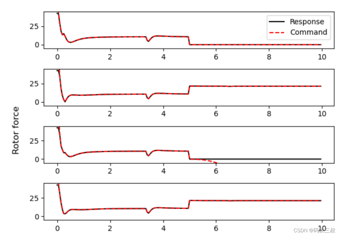
图2-10  绘制的两幅子图

2.3.7  基于自适应鲁棒滑模控制的仿真测试

文件test_AdaptiveISMC_linear.py实现了一个基于自适应鲁棒滑模控制（Adaptive Robust Sliding Mode Control）的线性四旋翼飞行器仿真环境。通过AdaptiveISMC_linear类来设计控制器，该控制器使用自适应技术来调整系统参数，以应对未知扰动和模型不确定性。仿真环境通过Copter_linear模型描述飞行器动力学，并提供了绘制仿真结果的功能。在仿真过程中，记录并绘制了飞行器的位置、速度、姿态角、角速度以及控制输入等关键信息，以评估控制器在不同飞行任务中的性能。

class Env(BaseEnv):
    def __init__(self):
        super().__init__(solver="odeint", max_t=10, dt=5, ode_step_len=100)
        self.plant = Copter_linear()
        ic = np.vstack((0, 0, 0, 0, 0, 0, 0, 0, 0, 0, 0, 0))
        pos_des0 = np.vstack((1, -1, -2))
        vel_des0 = np.vstack((0, 0, 0))
        angle_des0 = np.vstack((0, 0, 0))
        omega_des0 = np.vstack((0, 0, 0))
        ref0 = np.vstack((pos_des0, vel_des0, angle_des0, omega_des0))
        self.controller = AdaptiveISMC_linear(self.plant.J,
                                              self.plant.m,
                                              self.plant.g,
                                              self.plant.d,
                                              ic,
                                              ref0)

    def step(self):
        *_, done = self.update()
        return done

    def control_allocation(self, forces):
        rotors = np.linalg.pinv(self.plant.mixer.B).dot(forces)
        rotors = np.clip(rotors, 0, self.plant.rotor_max)
        return rotors

    def get_ref(self, t, x):
        pos_des = np.vstack((1, -1, -2))
        vel_des = np.vstack((0, 0, 0))
        # pos_des = np.vstack((cos(t), sin(t), -t))
        # vel_des = np.vstack((-sin(t), cos(t), -1))
        angle_des = np.vstack((0, 0, 0))
        omega_des = np.zeros((3, 1))
        ref = np.vstack((pos_des, vel_des, angle_des, omega_des))
        return ref

    def _get_derivs(self, t, x, p, gamma):
        ref = self.get_ref(t, x)
        K = np.array([[25, 20],
                      [100, 20],
                      [100, 20],
                      [25, 10]])
        Kc = np.vstack((10, 10, 10, 10))
        PHI = np.vstack([1] * 4)
        forces, sliding = self.controller.get_FM(x, ref, p, gamma, K, Kc, PHI, t)
        rotors = self.control_allocation(forces)
        return forces, rotors, ref, sliding

    def set_dot(self, t):
        x = self.plant.state
        p, gamma = self.controller.observe_list()
        forces, rotors, ref, sliding = self._get_derivs(t, x, p, gamma)
        self.plant.set_dot(t, rotors)
        self.controller.set_dot(x, ref, sliding)

    def logger_callback(self, i, t, y, *args):
        states = self.observe_dict(y)
        x_flat = self.plant.observe_vec(y[self.plant.flat_index])
        ctrl_flat = self.controller.observe_list(y[self.controller.flat_index])
        forces, rotors, ref, sliding = self._get_derivs(t, x_flat, ctrl_flat[0], ctrl_flat[1])
        return dict(t=t, **states, rotors=rotors, ref=ref, gamma=ctrl_flat[1], s=sliding)

def run():
    env = Env()
    env.logger = fym.logging.Logger("data.h5")
    env.reset()
    while True:
        env.render()
        done = env.step()
        if done:
            break
    env.close()

def exp1():
    run()

def exp1_plot():
    data = fym.logging.load("data.h5")

    fig = plt.figure()
    ax1 = fig.add_subplot(4, 1, 1)
    ax2 = fig.add_subplot(4, 1, 2, sharex=ax1)
    ax3 = fig.add_subplot(4, 1, 3, sharex=ax1)
    ax4 = fig.add_subplot(4, 1, 4, sharex=ax1)

    ax1.plot(data['t'], data['plant']['pos'].squeeze(), label="plant")
    ax1.plot(data["t"], data["ref"][:, 0, 0], "r--", label="plant (cmd)")
    ax1.plot(data["t"], data["ref"][:, 1, 0], "r--", label="y (cmd)")
    ax1.plot(data["t"], data["ref"][:, 2, 0], "r--", label="z (cmd)")
    ax2.plot(data['t'], data['plant']['vel'].squeeze())
    ax3.plot(data['t'], np.rad2deg(data['plant']['angle'].squeeze()))
    ax4.plot(data['t'], np.rad2deg(data['plant']['omega'].squeeze()))

    ax1.set_ylabel('Position [m]')
    ax1.legend([r'$x$', r'$y$', r'$z$'])
    ax1.grid(True)

    ax2.set_ylabel('Velocity [m/s]')
    ax2.legend([r'$u$', r'$v$', r'$w$'])
    ax2.grid(True)

    ax3.set_ylabel('Euler angle [deg]')
    ax3.legend([r'$phi$', r'$theta$', r'$psi$'])
    ax3.grid(True)

    ax4.set_ylabel('Angular Velocity [deg/s]')
    ax4.legend([r'$p$', r'$q$', r'$r$'])
    ax4.set_xlabel('Time [sec]')
    ax4.grid(True)

    plt.tight_layout()

    fig2 = plt.figure()
    ax1 = fig2.add_subplot(4, 1, 1)
    ax2 = fig2.add_subplot(4, 1, 2, sharex=ax1)
    ax3 = fig2.add_subplot(4, 1, 3, sharex=ax1)
    ax4 = fig2.add_subplot(4, 1, 4, sharex=ax1)

    ax1.plot(data['t'], data['rotors'].squeeze()[:, 0])
    ax2.plot(data['t'], data['rotors'].squeeze()[:, 1])
    ax3.plot(data['t'], data['rotors'].squeeze()[:, 2])
    ax4.plot(data['t'], data['rotors'].squeeze()[:, 3])

    ax1.set_ylabel('rotor1')
    ax1.grid(True)
    ax2.set_ylabel('rotor2')
    ax2.grid(True)
    ax3.set_ylabel('rotor3')
    ax3.grid(True)
    ax4.set_ylabel('rotor4')
    ax4.grid(True)
    ax4.set_xlabel('Time [sec]')

    plt.tight_layout()

    fig3 = plt.figure()
    ax1 = fig3.add_subplot(4, 1, 1)
    ax2 = fig3.add_subplot(4, 1, 2, sharex=ax1)
    ax3 = fig3.add_subplot(4, 1, 3, sharex=ax1)
    ax4 = fig3.add_subplot(4, 1, 4, sharex=ax1)

    ax1.plot(data['t'], data['gamma'].squeeze()[:, 0])
    ax2.plot(data['t'], data['gamma'].squeeze()[:, 1])
    ax3.plot(data['t'], data['gamma'].squeeze()[:, 2])
    ax4.plot(data['t'], data['gamma'].squeeze()[:, 3])

    ax1.set_ylabel('gamma1')
    ax1.grid(True)
    ax2.set_ylabel('gamma2')
    ax2.grid(True)
    ax3.set_ylabel('gamma3')
    ax3.grid(True)
    ax4.set_ylabel('gamma4')
    ax4.grid(True)
    ax4.set_xlabel('Time [sec]')

    plt.tight_layout()

    fig4 = plt.figure()
    ax1 = fig4.add_subplot(4, 1, 1)
    ax2 = fig4.add_subplot(4, 1, 2, sharex=ax1)
    ax3 = fig4.add_subplot(4, 1, 3, sharex=ax1)
    ax4 = fig4.add_subplot(4, 1, 4, sharex=ax1)

    ax1.plot(data['t'], data['s'].squeeze()[:, 0])
    ax2.plot(data['t'], data['s'].squeeze()[:, 1])
    ax3.plot(data['t'], data['s'].squeeze()[:, 2])
    ax4.plot(data['t'], data['s'].squeeze()[:, 3])

    ax1.set_ylabel('s1')
    ax1.grid(True)
    ax2.set_ylabel('s2')
    ax2.grid(True)
    ax3.set_ylabel('s3')
    ax3.grid(True)
    ax4.set_ylabel('s4')
    ax4.grid(True)
    ax4.set_xlabel('Time [sec]')
    plt.tight_layout()
    plt.show()

为节省本书篇幅，后面的测试文件test/test_AdaptiveISMC_nonlinear.py、test/test_ISMC_linear.py、test/test_ISMC_nonlinear.py、test/test_lqr.py不再讲解。

本项目已完结：

（2-3-1）位置控制算法：无人机运动控制系统（1）-CSDN博客

（2-3-2）位置控制算法：无人机运动控制系统（2）-CSDN博客

（2-3-3）位置控制算法：无人机运动控制系统——基于自适应反演滑模控制器的仿真测试-CSDN博客

（2-3-4）位置控制算法：无人机运动控制系统——基于非线性动力学和积分滑模控制的仿真测试-CSDN博客