（2-3-3）位置控制算法：无人机运动控制系统——基于自适应反演滑模控制器的仿真测试

2.3.5  基于自适应反演滑模控制器的仿真测试

文件test/fault_AISMC.py实现了一个基于非线性动力学模型的无人机飞行控制仿真环境，通过使用自适应反演滑模控制器（Adaptive Inverse Sliding Mode Control，AdaptiveISMC_nonlinear）对无人机进行控制，并引入了执行器故障模型以模拟实际飞行中可能发生的故障情况。最后可视化仿真结果，展示了无人机在控制算法下的轨迹、执行器状态、故障检测与隔离等信息，用于分析控制器对飞行器动态响应及故障情况的影响。

文件test/fault_AISMC.py的具体实现流程如下所示。

（1）函数Env.init()用于初始化仿真环境，包括定义执行器故障（actuator_faults）、初始条件（ic）、参考轨迹（ref0）以及创建无人机模型（Copter_nonlinear）、执行器故障检测与隔离模块（FDI）和自适应反演滑模控制器（AdaptiveISMC_nonlinear）。

class Env(BaseEnv):
    def __init__(self):
        super().__init__(solver="odeint", max_t=20, dt=10, ode_step_len=100)
        # Define faults
        self.actuator_faults = [
            LoE(time=5, index=0, level=0.0),
            # LoE(time=10, index=3, level=0.3)
        ]
        # Define initial condition and reference at t=0
        ic = np.vstack((0, 0, 0, 0, 0, 0, 1, 0, 0, 0, 0, 0, 0))
        ref0 = np.vstack((1, -1, -2, 0, 0, 0, 1, 0, 0, 0, 0, 0, 0))
        # Define agents
        self.plant = Copter_nonlinear()
        self.n = self.plant.mixer.B.shape[1]
        self.fdi = FDI(numact=self.n)
        self.controller = AdaptiveISMC_nonlinear(self.plant.J,
                                                 self.plant.m,
                                                 self.plant.g,
                                                 self.plant.d,
                                                 ic,
                                                 ref0)

（2）函数Env.get_ref(t, x)的功能是根据当前时间 t 和状态 x 计算参考轨迹 ref，包括期望位置、速度、姿态和角速度。

    def get_ref(self, t, x):
        pos_des = np.vstack((1, -1, -2))
        vel_des = np.vstack((0, 0, 0))
        quat_des = np.vstack((1, 0, 0, 0))
        omega_des = np.zeros((3, 1))
        ref = np.vstack((pos_des, vel_des, quat_des, omega_des))
        return ref

（3）函数Env._get_derivs(t, x, p, gamma, effectiveness)的功能根据当前时间 t、状态 x、控制参数 p、滑模变量 gamma 和执行器效应性 effectiveness 计算执行器指令、执行器输出、作用在飞行器上的力和滑模变量。

    def _get_derivs(self, t, x, p, gamma, effectiveness):
        ref = self.get_ref(t, x)
        forces, sliding = self.controller.get_FM(x, ref, p, gamma, t)
        # Controller
        Bf = self.plant.mixer.B * effectiveness
        L = np.diag(effectiveness)
        rotors_cmd = np.linalg.pinv(Bf.dot(L)).dot(forces)
        rotors = np.clip(rotors_cmd, 0, self.plant.rotor_max)
        return rotors_cmd, rotors, forces, ref, sliding

（4）函数Env.set_dot(t的功能根据当前时间 t 更新仿真状态的导数，包括计算执行器指令、执行器输出和作用在飞行器上的力，并更新控制器和飞行器的状态。

    def set_dot(self, t):
        x = self.plant.state
        p, gamma = self.controller.observe_list()
        effectiveness = np.array([1.] * self.n)
        for act_fault in self.actuator_faults:
            effectiveness = act_fault.get_effectiveness(t, effectiveness)
        rotors_cmd, rotors, forces, ref, sliding = \
            self._get_derivs(t, x, p, gamma, effectiveness)

        self.plant.set_dot(t, rotors)
        self.controller.set_dot(x, ref, sliding)

（5）函数Env.logger_callback(i, t, y, *args)是仿真过程中的日志记录回调函数，用于提取并返回包括时间 t、飞行器状态 x、执行器指令、执行器输出、参考轨迹、滑模变量和作用在飞行器上的力等信息的字典。

    def logger_callback(self, i, t, y, *args):
        states = self.observe_dict(y)
        x_flat = self.plant.observe_vec(y[self.plant.flat_index])
        ctrl_flat = self.controller.observe_list(y[self.controller.flat_index])
        x = states["plant"]
        effectiveness = np.array([1.] * self.n)
        for act_fault in self.actuator_faults:
            effectiveness = act_fault.get_effectiveness(t, effectiveness)
        rotors_cmd, rotors, forces, ref, sliding = \
            self._get_derivs(t, x_flat, ctrl_flat[0], ctrl_flat[1], effectiveness)

        return dict(t=t, x=x, rotors=rotors, rotors_cmd=rotors_cmd,
                    ref=ref, gamma=ctrl_flat[1], forces=forces)

（6）函数exp1_plot()用于绘制仿真结果的多个子图，包括飞行器执行器指令与实际输出的对比、期望轨迹与实际轨迹的对比、执行器故障检测与隔离滑模变量的演变，以及在执行器故障发生时的标注。通过可视化展示飞行器的动态响应和控制性能，有助于分析控制系统的稳定性和鲁棒性。

def exp1_plot():
    data = fym.logging.load("case3_A.h5")
    print(data.keys())
    # Rotor
    plt.figure()
    ax = plt.subplot(411)
    plt.plot(data["t"], data["rotors"][:, 0], "k-", label="Response")
    plt.plot(data["t"], data["rotors_cmd"][:, 0], "r--", label="Command")
    plt.ylim([-5.1, 45])
    plt.legend()

    plt.subplot(412, sharex=ax)
    plt.plot(data["t"], data["rotors"][:, 1], "k-")
    plt.plot(data["t"], data["rotors_cmd"][:, 1], "r--")
    plt.ylim([-5.1, 45])

    plt.subplot(413, sharex=ax)
    plt.plot(data["t"], data["rotors"][:, 2], "k-")
    plt.plot(data["t"], data["rotors_cmd"][:, 2], "r--")
    plt.ylim([-5.1, 45])

    plt.subplot(414, sharex=ax)
    plt.plot(data["t"], data["rotors"][:, 3], "k-")
    plt.plot(data["t"], data["rotors_cmd"][:, 3], "r--")
    plt.ylim([-5.1, 45])

    plt.gcf().supxlabel("Time, sec")
    plt.gcf().supylabel("Rotor force")
    plt.tight_layout()

    plt.figure()

    ax = plt.subplot(411)
    plt.plot(data["t"], data["ref"][:, 0, 0], "r-", label="x (cmd)")
    plt.plot(data["t"], data["x"]["pos"][:, 0, 0], label="x")

    plt.plot(data["t"], data["ref"][:, 1, 0], "r--", label="y (cmd)")
    plt.plot(data["t"], data["x"]["pos"][:, 1, 0], label="y")

    plt.plot(data["t"], data["ref"][:, 2, 0], "r-.", label="z (cmd)")
    plt.plot(data["t"], data["x"]["pos"][:, 2, 0], label="z")
    plt.legend(loc='center left', bbox_to_anchor=(1, 0.5))

    plt.axvspan(5, 5.042, alpha=0.2, color="b")
    plt.axvline(5.042, alpha=0.8, color="b", linewidth=0.5)
    plt.annotate("Rotor 0 fails", xy=(5, 0), xytext=(5.5, 0.5),
                 arrowprops=dict(arrowstyle='->', lw=1.5))

    plt.subplot(412, sharex=ax)
    plt.plot(data["t"], data["x"]["vel"].squeeze())
    plt.legend([r'$u$', r'$v$', r'$w$'], loc='center left', bbox_to_anchor=(1, 0.5))

    plt.axvspan(5, 5.042, alpha=0.2, color="b")
    plt.axvline(5.042, alpha=0.8, color="b", linewidth=0.5)
    plt.annotate("Rotor 0 fails", xy=(5, 0), xytext=(5.5, 0.5),
                 arrowprops=dict(arrowstyle='->', lw=1.5))

    plt.subplot(413, sharex=ax)
    plt.plot(data["t"], data["x"]["quat"].squeeze())
    plt.legend([r'$q0$', r'$q1$', r'$q2$', r'$q3$'])
    # plt.plot(data["t"], np.transpose(quat2angle(np.transpose(data["x"]["quat"].squeeze()))))
    # plt.legend([r'$psi$', r'$theta$', r'$phi$'], loc='center left', bbox_to_anchor=(1, 0.5))
    plt.axvspan(5, 5.042, alpha=0.2, color="b")
    plt.axvline(5.042, alpha=0.8, color="b", linewidth=0.5)
    plt.annotate("Rotor 0 fails", xy=(5, 0), xytext=(5.5, 0.5),
                 arrowprops=dict(arrowstyle='->', lw=1.5))

    plt.subplot(414, sharex=ax)
    plt.plot(data["t"], data["x"]["omega"].squeeze())
    plt.legend([r'$p$', r'$q$', r'$r$'], loc='center left', bbox_to_anchor=(1, 0.5))
    plt.axvspan(5, 5.042, alpha=0.2, color="b")
    plt.axvline(5.042, alpha=0.8, color="b", linewidth=0.5)
    plt.annotate("Rotor 0 fails", xy=(5, 0), xytext=(5.5, 0.5),
                 arrowprops=dict(arrowstyle='->', lw=1.5))

    # plt.xlabel("Time, sec")
    # plt.ylabel("Position")
    # plt.legend(loc="right")
    plt.tight_layout()

    plt.figure()

    ax = plt.subplot(411)
    plt.plot(data['t'], data['gamma'].squeeze()[:, 0])
    plt.ylabel(r'$-\hat{h_{1}}$')
    plt.grid(True)
    plt.axvspan(5, 5.042, alpha=0.2, color="b")
    plt.axvline(5.042, alpha=0.8, color="b", linewidth=0.5)
    plt.annotate("Rotor 0 fails", xy=(5, 0), xytext=(5.5, 0.5),
                 arrowprops=dict(arrowstyle='->', lw=1.5))

    plt.subplot(412, sharex=ax)
    plt.plot(data['t'], data['gamma'].squeeze()[:, 1])
    plt.ylabel(r'$\hat{h_{2}}$')
    plt.grid(True)
    plt.axvspan(5, 5.042, alpha=0.2, color="b")
    plt.axvline(5.042, alpha=0.8, color="b", linewidth=0.5)
    plt.annotate("Rotor 0 fails", xy=(5, 0), xytext=(5.5, 0.5),
                 arrowprops=dict(arrowstyle='->', lw=1.5))

    plt.subplot(413, sharex=ax)
    plt.plot(data['t'], data['gamma'].squeeze()[:, 2])
    plt.ylabel(r'$\hat{h_{3}}$')
    plt.grid(True)
    plt.axvspan(5, 5.042, alpha=0.2, color="b")
    plt.axvline(5.042, alpha=0.8, color="b", linewidth=0.5)
    plt.annotate("Rotor 0 fails", xy=(5, 0), xytext=(5.5, 0.5),
                 arrowprops=dict(arrowstyle='->', lw=1.5))

    plt.subplot(414, sharex=ax)
    plt.plot(data['t'], data['gamma'].squeeze()[:, 3])
    plt.ylabel(r'$\hat{h_{4}}$')
    plt.grid(True)
    plt.axvspan(5, 5.042, alpha=0.2, color="b")
    plt.axvline(5.042, alpha=0.8, color="b", linewidth=0.5)
    plt.annotate("Rotor 0 fails", xy=(5, 0), xytext=(5.5, 0.5),
                 arrowprops=dict(arrowstyle='->', lw=1.5))
    plt.xlabel("Time [sec]")

    plt.tight_layout()

    # fig4 = plt.figure()
    # ax1 = fig4.add_subplot(4, 1, 1)
    # ax2 = fig4.add_subplot(4, 1, 2, sharex=ax1)
    # ax3 = fig4.add_subplot(4, 1, 3, sharex=ax1)
    # ax4 = fig4.add_subplot(4, 1, 4, sharex=ax1)

    # ax1.plot(data['t'], data['forces'].squeeze()[:, 0])
    # ax2.plot(data['t'], data['forces'].squeeze()[:, 1])
    # ax3.plot(data['t'], data['forces'].squeeze()[:, 2])
    # ax4.plot(data['t'], data['forces'].squeeze()[:, 3])

    # ax1.set_ylabel('F')
    # ax1.grid(True)
    # ax2.set_ylabel('M1')
    # ax2.grid(True)
    # ax3.set_ylabel('M2')
    # ax3.grid(True)
    # ax4.set_ylabel('M3')
    # ax4.grid(True)
    # ax4.set_xlabel('Time [sec]')
    # plt.tight_layout()
    plt.show()

执行后将回执多个子图，如图2-8所示。

1. 执行器输出与指令对比图：包含四个子图，每个子图对应飞行器的一个执行器，展示了执行器的实际输出与控制器指令之间的对比，以评估执行器的性能。
2. 控制系统状态与期望轨迹对比图：包含四个子图，分别展示了飞行器的位置、速度、姿态以及角速度的实际状态与期望轨迹之间的对比，以评估控制系统的跟踪性能。
3. 执行器故障检测与隔离滑模变量演变图： 展示了执行器故障检测与隔离系统的滑模变量在时间上的演变，以分析故障检测与隔离性能。

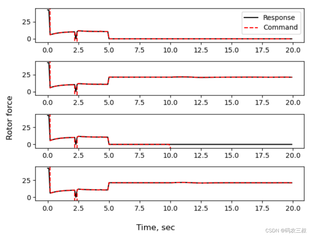
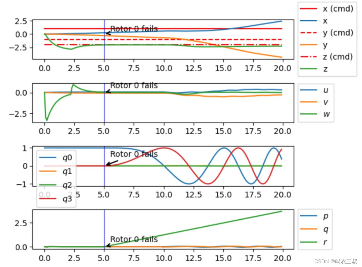
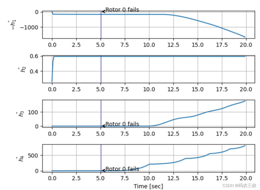
图2-9  绘制的子图

未完待续