论文笔记|Spatial Pyramid Pooling in Deep Convolutional Networks for Visual Recognition

Authors

Kaiming He, Xiangyu Zhang, Shaoqing Ren, and Jian Sun

何恺明

Abstract

Existing CNNs require a fixed-size input image.This requirement may reduce the recongnition accuracy for the image or sub-image of an arbitray size/scale. In this work, SPP-net can generate a fixed-length represention regardless of image szie/scale. In the object detection respect, this method aviods repeatedly computing the convolutional features, and 24-102x faster than R-CNN.

1 Introduction

A CNN mainly consists of two parts: convolutional layers and fully-connected layers. (btw output feature maps represent the spatial arrangement of the activations) it is fixed-size/length is needed by the fc layers rather than the convolutional layers. In this paper , an SPP layer was added on the top of the last convolutional layer .
SPP,as an extension of the BoW, it has some remarkable properties for CNNs:
1. generates a fixed-length
2. uses multi-level spatial bins, robust
3. can pool features extracted at variable scales

# for spp and wob
K. Grauman and T. Darrell, “The pyramid match kernel: Discriminative classification with sets of image features,” in
ICCV, 2005.
 S. Lazebnik, C. Schmid, and J. Ponce, “Beyond bags of features: Spatial pyramid matching for recognizing natural scene categories,” in CVPR, 2006.

SPPnet allows us to feed images with varying sizes, and experiments show that multi-size training converges just as the traditional single-size training, and lead to better testing accuracy.

SPP impoves four different CNN architectures,it might improve more sophisticated convolutinal architectures.

About object detection, we can run the convolutional layers only once and then extract features on the feature maps by spp-net. with the recent fast proposal method of EdgeBoxes, our system takes 0.5 seconds processing an image.

2 Deep networks with spp

2.1 feature map

the convolutinal layers use sliding filters, and their outputs have roughly the same aspect ratio as the inputs,so the feature map involve not only the strength of the responses, but also their spatial positions.

2.2 trainin the network

2.2.1 single-size training

spp layer windowsize=$\lceil a/n \rceil$, stride =$\lfloor a/n \rfloor$

2.2.2 multi-size training

we consider a set of predefined sizes(180x180,224,224),we resize the 224x224 region to 180 x 180

Note that the above single/ multi-size solutions are for training only, at the testing stage, it is straightforward to apply on images of any size.

3 SPP-net for image classification

3.1 Experiments on ImageNet 2012 classification

3.1.1 baseline architectures

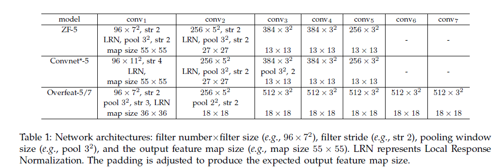
the advangetages of spp are independent of the cnn architectures used. we show spp improves the accuracy of all these 4 architectures in table 1.

3.1.2 multi-level pooling improves accuracy

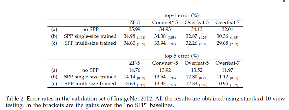
In table 2 we show the results using single-size training with the spp layer replace the previous regular pooling layer.

It is worth noticing that the gain of multi-level pooling is brought by the it’s robust, which to the variance in object deformations and spatial layout.

3.1.3 multi-size training improves accuracy

Table 2 (c) shows the multi-size training.

3.1.4 full-image representations improve accuracy

full-image: min(w,h)=256
single view: center 224x224 crop
The comparisions are in table 3, and it shows that even though our network is trained using square images only, it generalizes well to other aspect rations:

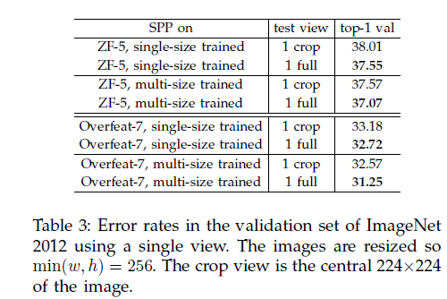
comparing Table2 and 3 ,we find that the combination of multiple view is substantially better than the single full-image view.
Good merits of full-image representations:
1. even for the combination of dozens of views, 2 additional full-image views(flipping) can still boost the accuracy by about 0.2%
2. full-image view is methodologically consistent with the traditional methods.
3. in other applications such as image retrieval an image representation, rather than a classification score , is required for similarity ranking. A full-image representation can be preferred.

# image retrieval
H. Jegou, F. Perronnin, M. Douze, J. Sanchez, P. Perez, and
C. Schmid, “Aggregating local image descriptors into compact
codes,” TPAMI, vol. 34, no. 9, pp. 1704–1716, 2012.

3.1.5 Multi-view testing on feature maps

On the testing stage, we resize an image so min(w,h)=s (e.g.s=256), for the usage of flipped views, we also compute the feature maps of the flipped image. Given any view in the image, we map this window to the feature maps(the way of mapping is in Appendix), and use SPP to pool the feature from the window( Figure 5), then the features are fed fed into the fc layers to compute the scores(averaged for the final prediction)

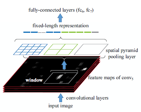
for the standard 10-veiw, we use s=256, views 224 on the center or corner, experiments show that top-5 error of the 10-view prediction on feature maps is within 0.1% around the original 10-view prediction on image crops.
extract multiple views from multiple scales:
we resize the image to six scales, and use 18 views for each scale(1center, 4corner,4middle, flipping), then there are 6x18-12(s=224)=96, reduce the top5 error from 10.95%->9.36%, Combining the two full-image views ,—>9.14%

3.2 voc 2007

We need re-train SVm classifiers, in the svm training, we intentionally do not use any data augmentation(flip/multi-view),$l_2$-normalize the features for svm training.

s=392 gives the best result, mainly bacause the objects occupy smaller regions in voc2007,but larger in ImageNet.

3.3 caltech 101

The spp layer are better, this is possibly because the object categories in Caltech101 are less related to those in ImageNet,but the scale is same.

4 Object detection

We only fine-tune the fully-connetcted layers, also use bounding-box regression.
can be improved by multi-scale feature extraction.

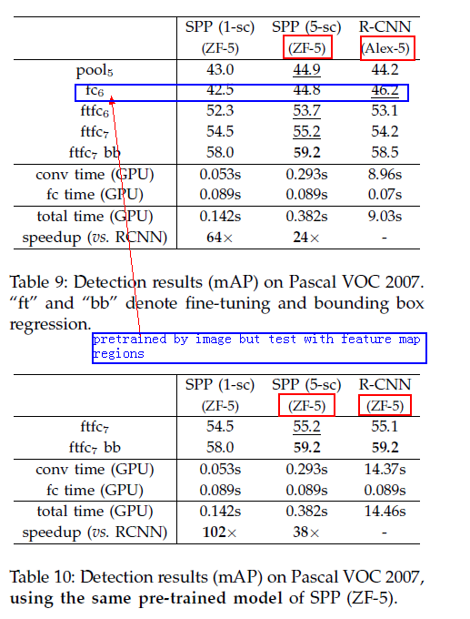
EdegeBox 0.2s / an image ,Selective Search 1-2 s/an image,
train:EB+SS,testEB—>56.3%>55.2%( all step 0.5s)

4.4 Model combination

Pre-train another network using same structure but **different randoom initialization**s.Then:
1. score all candidate windows on the test image.
2. perform non-maximum suppression on the union of the two sets of candidata windows.
3. mAP is boosted to 60.9%!

4.5 ILSVRC 2014 Detection

Interestingly, even if the amount of training data do not increas, training a network of more catefories boosts the feature quality.
six similar models –>35.11%
winning result is 37.21% from NUS(（National University of Singapore), which uses contextual information

Appendix

a Mean subtration

Warp the 224x224 mean image to the desired size and then subtract it. In pascal voc 2007, caltech101, we use the constant mean 128.

b Pooling bins

Denote the width and height of the conv5 feature maps as w and h, For a pyramid level with nxn bins, the (i,j)th bin is the range of $[\lceil \frac{i-1}{n}w \rceil ,\lfloor \frac{i}{n}w \rfloor ]\times[\lceil \frac{i-1}{n}h \rceil ,\lfloor \frac{i}{n}h \rfloor ]$

c Mapping a window to feature maps

filter size –>f
pad $\lfloor f/2 \rfloor$ for a layer
image domain –>(x,y)
response centered –>(x’,y’)
$x'_{top}=\lfloor x/s \rfloor+1$
$x'_{bottom}=\lceil x/s \rceil-1$

conclusion