论文笔记 | OverFeat: Integrated Recognition, Localization and Detection using Convolutional Networks

Author

Pierre Sermanet David Eigen Xiang Zhang Michael Mathieu Rob Fergus Yann LeCun

Pierre Sermanet

Abstract

We show how a multi-scale and sliding window approach can be implemented in a ConvNet. We also introduce a novel approach to localization by learning to predict boundaries. Bounding boxes are then accumulated rather than suppressed in order to increase detection confidence.

3 Classification

Our classification architecture is similar to the Krizhevsky’s network, however, we inprove on the network design and inference step.

3.1 Model Design and training

Each image is downsampled so that the smallest dimension is 256 pixels. We than extract 5 crops (random 221x221) and then horizontal flips.
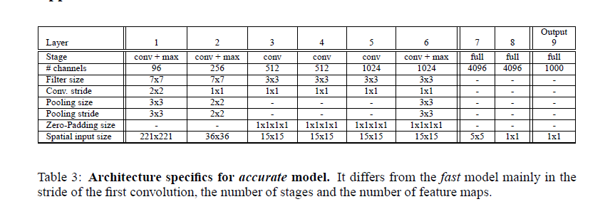
The architecture sizes are detailed in the followed tables:


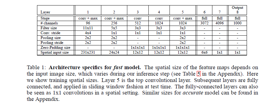
Layers 1-5 are similar to Kriz’s, using relu and max pooling, but with the following differences:
1. no contrast normalization is used(???)
2. pooling are non-overlapping
3. has larger 1st,2nd layer feature maps.(stride4->2)

3.3 Multi-scale classification

Multi-view voting:1) can ignore many regions of the image 2)computattionally redundant when views overlap 3)one single scale. So MULTISCALE CALSSIFICATION


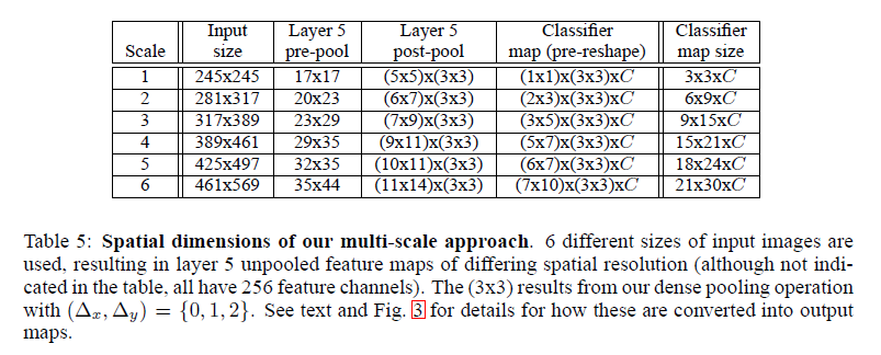
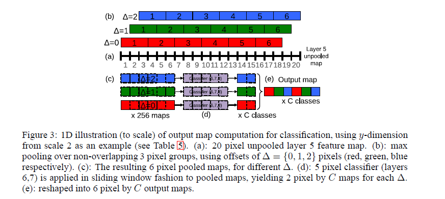
1. For a single image, at a given scale, we start with the unpooled layer 5 feature maps.
2. Each of the unpooled maps undergoes a 3x3 non-overlapping pooling operation, repeated 3x3 times (for x and y)(fig.3)
3. This produces a set of pooled feature maps
4. Classifier(filter) has a fixed input size(5x5), and is applied in sliding-window fashion to the pooled maps, yielding C dimensionsal output maps.
5. The output maps for different combinations are reshaped into 3d output maps
The procedure above is repeated for the horizontally flipped version of each image.
We than produce the final classification by:
1. taking the spatial max for each class, at each scale and flip
2. averaging the resulting C-d vectors from different scales and flips
3. taking the top1 or top5 elements from the mean class vector.
The exhaustive pooling scheme( single pixel shifts($\Delta_x,\Delta_y$)) ensures that we can obtain fine alignment between the classifier and the object.

3.5 efficiency

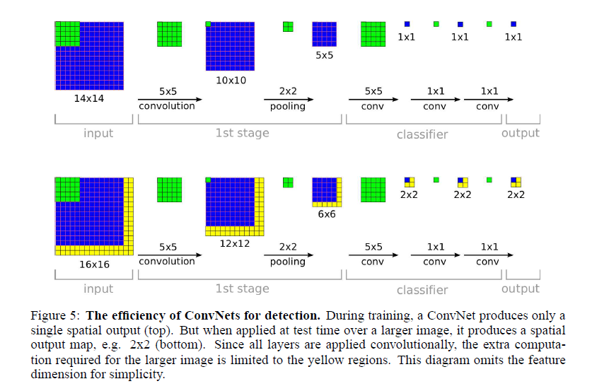
Note that the last layers of our architecture are fully connected linear layers, At test time, layers are effectively replaced by convolution operations with kernels of 1x1 spatial extent. The entire ConvNet is then simply a sequence of convolutions, maxpooling and thresholding operations exclusively.

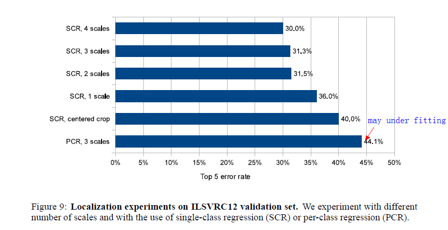
4 Localization

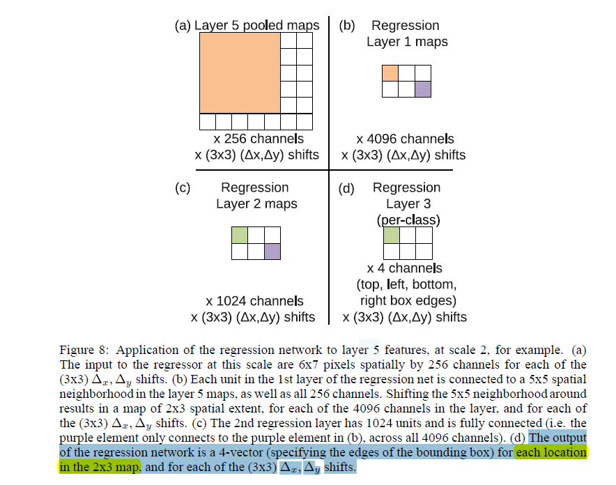
Replace the classifier layers by a regression network and train it to predict object bounding boxes at each spatial location and scale. The we combine the regression predictions together.

4.2 regressor training

4.3 combining predictions

1. top k classes for each scale–>$C_s$
2. bounding boxes for $C_s$–>$B_s$
3. $\cup_s B_s \rightarrow B$
4. $(b'_1,b'_2)=argmin_{b_1\neq b_2}match\_ score(b_1,b_2)$
5. for $(match\_score(b'_1,b'_2)<t)$:
   B=B{$b_1',b'_2$}$\cup box\_merge(b_1',b_2')$
   match_score=sum of the distance between centers of the two bounding boxes and the intersection area of the boxes
   box_merge= average of the bounding boxes’s coordinates.
   

6 discussion

Our approach might still be improved in several ways:
1. For localization, we are not currently back-propping through the whole network
2. IoU can take the place of l2 loss in our approach
3. Alternate parameterizations of the bounding box may help to decorrelate the outputs, which will aid network training.

7 conclusion