02_graph 图分类任务

mingqian_chu

已于 2024-05-29 15:58:59 修改

阅读量23

点赞数

分类专栏： # 图神经网络文章标签：分类数据挖掘人工智能

于 2024-05-15 16:39:23 首次发布

原文链接：pyG.com

版权

图神经网络专栏收录该内容

21 篇文章 1 订阅

订阅专栏

原文出自PYG 官方教程，
https://pytorch-geometric.readthedocs.io/en/latest/get_started/colabs.html；

说完节点分类的任务, 接下来就该介绍图分类任务了.

下载PyG库

# Install required packages.

import os
import torch
os.environ['TORCH'] = torch.__version__
print(torch.__version__)

!pip install -q torch-scatter -f https://pytorch-geometric.com/whl/torch-1.10.0+cu113.html
!pip install -q torch-sparse -f https://pytorch-geometric.com/whl/torch-1.10.0+cu113.html
!pip install -q git+https://github.com/rusty1s/pytorch_geometric.git

使用图神经网络来分类图

图分类 (Graph classification) 指的是对于已知的图数据集, 基于一些结构图的属性, 分类整张图的任务. 因此, 我们需要嵌入整张图, 并且使它们在某些任务下是线性可分的.

在这里插入图片描述

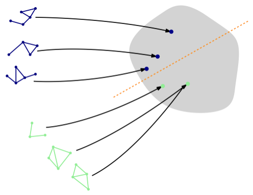
图分类中, 最常见的任务是 分子性质预测 (molecular property prediction), 其中一个分子被表达成一张图. 举个例子, 任务可以是推断一个分子是否抑制HIV病毒的复制. 多特蒙德工业大学收集了广泛的图分类数据集, 取名为**TUDatasets**. 在PyG中, 我们可以通过 [torch_geometric.datasets.TUDataset] 来获取这个数据集. 让我们来加载 MUTAG 数据集:

import torch
from torch_geometric.datasets import TUDataset

dataset = TUDataset(root='data/TUDataset', name='MUTAG')

print()
print(f'Dataset: {dataset}:')
print('====================')
print(f'Number of graphs: {len(dataset)}')
print(f'Number of features: {dataset.num_features}')
print(f'Number of classes: {dataset.num_classes}')

data = dataset[0]  # Get the first graph object.

print()
print(data)
print('=============================================================')

# Gather some statistics about the first graph.
print(f'Number of nodes: {data.num_nodes}')
print(f'Number of edges: {data.num_edges}')
print(f'Average node degree: {data.num_edges / data.num_nodes:.2f}')
print(f'Has isolated nodes: {data.has_isolated_nodes()}')
print(f'Has self-loops: {data.has_self_loops()}')
print(f'Is undirected: {data.is_undirected()}')

输出结果:

Downloading https://www.chrsmrrs.com/graphkerneldatasets/MUTAG.zip
Extracting data/TUDataset/MUTAG/MUTAG.zip
Processing...

Dataset: MUTAG(188):
====================
Number of graphs: 188
Number of features: 7
Number of classes: 2

Data(edge_index=[2, 38], x=[17, 7], edge_attr=[38, 4], y=[1])
=============================================================
Number of nodes: 17
Number of edges: 38
Average node degree: 2.24
Has isolated nodes: False
Has self-loops: False
Is undirected: True
Done!

这个数据集提供 188张不同的图, 我们的任务是分类每张图到两个类别中的一个.

通过检查数据集的第一个图对象, 我们可以发现它有 17个节点 (每个节点有 7维的特征向量), 和 38条边 (平均节点出入度数 38/17=2.24), 每张图都有 一个图标签 y=[1]. 另外, 每条边还有额外的 4维边特征 (edge feature) edge_attr=[38, 4]. 但是, 为了让本教程足够简单, 我们不会使用这些额外特征.

PyG 提供一些便利函数来帮助我们更好地处理图数据集, 例如, 我们可以洗牌 (shuffle) 数据集, 并使用前150个图作为训练集, 其余的用作测试:

torch.manual_seed(12345)
dataset = dataset.shuffle()

train_dataset = dataset[:150]
test_dataset = dataset[150:]

print(f'Number of training graphs: {len(train_dataset)}')
print(f'Number of test graphs: {len(test_dataset)}')

输出结果:

Number of training graphs: 150
Number of test graphs: 38

图的小批量 (mini-batching) 训练

既然在图分类数据集中的单张图都比较小, 我们可以在输入到 GNN 之前, 对图进行批处理, 这样可以保证充分 GPU 的利用率. 在图像或语言领域, 这一过程通常通过将每个样例 缩放 (rescaling) 或填充 (padding) 为一组形状相等的数据来实现 (这样输入数据就多了一个额外的维度). 这个维度的长度等于在小批量中的样本个数, 我们通常称其为 batch_size.

但是, 对于GNN来说, 上述的两种方法都不可行, 或者说可能会导致不必要的内存消耗. 因此, PyG使用另一种方法优化, 在这里，邻接矩阵以对角线方式堆叠（创建一个包含多个孤立子图的巨型图），节点和目标特征在节点维度中简单地连接起来：

在这里插入图片描述

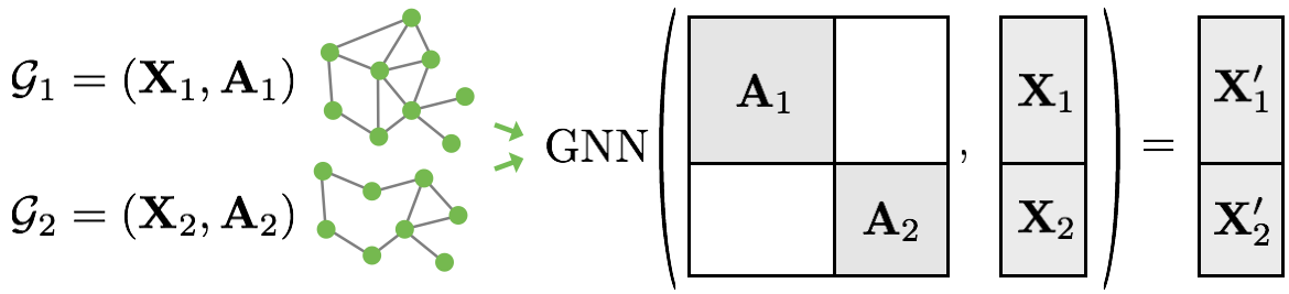
此程序与其他批处理程序相比有一些关键的优点:

依赖于消息传递方案的 GNN 运算符不需要修改，因为消息不会在属于不同图的两个节点之间交换。

There is no computational or memory overhead since adjacency matrices are saved in a sparse fashion holding only non-zero entries, i.e., the edges.
2. 没有计算或内存开销，因为邻接矩阵以稀疏方式保存，仅包含非零条目，即边缘。

通过 [torch_geometric.data.DataLoader] 类, PyG会自动地处理, 构建多个子图成一个批量的大图.

from torch_geometric.loader import DataLoader

train_loader = DataLoader(train_dataset, batch_size=64, shuffle=True)
test_loader = DataLoader(test_dataset, batch_size=64, shuffle=False)

for step, data in enumerate(train_loader):
    print(f'Step {step + 1}:')
    print('=======')
    print(f'Number of graphs in the current batch: {data.num_graphs}')
    print(data)
    print()

输出结果:

Step 1:
=======
Number of graphs in the current batch: 64
Batch(edge_attr=[2560, 4], edge_index=[2, 2560], x=[1154, 7], y=[64], batch=[1154], ptr=[65])

Step 2:
=======
Number of graphs in the current batch: 64
Batch(edge_attr=[2454, 4], edge_index=[2, 2454], x=[1121, 7], y=[64], batch=[1121], ptr=[65])

Step 3:
=======
Number of graphs in the current batch: 22
Batch(edge_attr=[980, 4], edge_index=[2, 980], x=[439, 7], y=[22], batch=[439], ptr=[23])

这里我们使用64的 batch_size, 这样我们会有3个小批量, 也就是包含 2 * 64 + 22 = 150 张图.

Furthermore, each Batch object is equipped with a batch vector, which maps each node to its respective graph in the batch:
此外，每个 Batch 对象都配备了一个 batch 向量，该向量将每个节点映射到批处理中各自的图形：

${batch} = [0, ..., 0, 1, ..., 1, 2, ...]$

训练 GNN

要训练一个GNN来进行图分类, 我们通常需要以下步骤:

Embed each node by performing multiple rounds of message passing
通过执行多轮消息传递来嵌入每个节点
Aggregate node embeddings into a unified graph embedding (readout layer)
将节点嵌入聚合到统一的图形嵌入（读出层）中
Train a final classifier on the graph embedding
在图嵌入上训练最终分类器

文献中已有很多不同的 读出层, 但是最常用的只是简单地利用了节点嵌入的优势:

$\mathbf{x_{\mathcal{G}}} = \frac{1}{|\mathcal{V}|} \sum_{v \in \mathcal{V}} x_v^{(L)}$

PyG也同样提供这一读出层 [torch_geometric.nn.global_mean_pool],

该函数的输入为小批量内所有节点的节点嵌入和赋值向量 batch 来为批量内的每张图计算图嵌入 (形状为 [batch_size, hidden_channels]).

PyTorch Geometric 通过 torch_geometric.nn.global_mean_pool 提供此功能，它接受小批量中所有节点的节点嵌入和赋值向量 batch ，以计算批处理中每个图形大小 [batch_size, hidden_channels] 的图形嵌入。

将GNN应用于图分类任务的最终架构如下所示:

from torch.nn import Linear
import torch.nn.functional as F
from torch_geometric.nn import GCNConv
from torch_geometric.nn import global_mean_pool


class GCN(torch.nn.Module):
    def __init__(self, hidden_channels):
        super(GCN, self).__init__()
        torch.manual_seed(12345)
        self.conv1 = GCNConv(dataset.num_node_features, hidden_channels)
        self.conv2 = GCNConv(hidden_channels, hidden_channels)
        self.conv3 = GCNConv(hidden_channels, hidden_channels)
        self.lin = Linear(hidden_channels, dataset.num_classes)

    def forward(self, x, edge_index, batch):
        # 1. Obtain node embeddings 
        x = self.conv1(x, edge_index)
        x = x.relu()
        x = self.conv2(x, edge_index)
        x = x.relu()
        x = self.conv3(x, edge_index)

        # 2. Readout layer
        x = global_mean_pool(x, batch)  # [batch_size, hidden_channels]

        # 3. Apply a final classifier
        x = F.dropout(x, p=0.5, training=self.training)
        x = self.lin(x)
        
        return x

model = GCN(hidden_channels=64)
print(model)

输出结果:

GCN(
  (conv1): GCNConv(7, 64)
  (conv2): GCNConv(64, 64)
  (conv3): GCNConv(64, 64)
  (lin): Linear(in_features=64, out_features=2, bias=True)
)

在我们应用最后的分类器之前, 我们使用 [GCNConv] 和 ReLU(x)=max(x,0)激活, 来获得本地的节点嵌入, 现在让我们来训练这个网络:

model = GCN(hidden_channels=64)
optimizer = torch.optim.Adam(model.parameters(), lr=0.01)
criterion = torch.nn.CrossEntropyLoss()

def train():
    model.train()
    
    for data in train_loader:  # Iterate in batches over the training dataset.
        out = model(data.x, data.edge_index, data.batch)  # Perform a single forward pass.
        loss = criterion(out, data.y)  # Compute the loss.
        loss.backward()  # Derive gradients.
        optimizer.step()  # Update parameters based on gradients.
        optimizer.zero_grad()  # Clear gradients.

def test():
    model.eval()
    
    correct = 0
    for data in test_loader:  # Iterate in batches over the training/test dataset.
        out = model(data.x, data.edge_index, data.batch)  
        pred = out.argmax(dim=1)  # Use the class with highest probability.
        correct += int((pred == data.y).sum())  # Check against ground-truth labels.
    return correct / len(loader.dataset)  # Derive ratio of correct predictions.

for epoch in range(1, 171):
    train()
    train_acc = test(train_loader)
    test_acc = test(test_loader)
    print(f'Epoch: {epoch:03d}, Train Acc: {train_acc:.4f}, Test Acc: {test_acc:.4f}')

输出结果:

Epoch: 001, Train Acc: 0.6467, Test Acc: 0.7368
...
Epoch: 050, Train Acc: 0.7667, Test Acc: 0.8158
...
Epoch: 100, Train Acc: 0.7733, Test Acc: 0.7895
...
Epoch: 150, Train Acc: 0.7800, Test Acc: 0.7895
...
Epoch: 170, Train Acc: 0.8000, Test Acc: 0.7632

不难发现, 我们的模型获得了大概 76%的测试准确度. 我们还可以观察到一些准确性波动, 这事因为我们的数据集比较小, 只有38个测试图, 一旦数据集增大, 这种波动通常就会消失.

课后作业

我们可以做得更好吗? 有不少的论文指出[1][2], 应用领域归一化 (neighborhood normalization) 降低了GNN在区分某些图结构时的表达性.

Morris 等提出的方法[2]完全避免了领域归一化, 并且为了保留中心节点的信息, 他们添加了一个简单的残差连接 (skip-connection) 到 GNN层中:

$\mathbf{x}_v^{(\ell+1)} = \mathbf{W}^{(\ell + 1)}_1 \mathbf{x}_v^{(\ell)} + \mathbf{W}^{(\ell + 1)}_2 \sum_{w \in \mathcal{N}(v)} \mathbf{x}_w^{(\ell)}$

在PyG中, 这一层叫做 [GraphConv]. 试试使用GraphConv来替换GCNConv. 我们应该能得到接近82%的测试准确度.

from torch_geometric.nn import GraphConv


class GNN(torch.nn.Module):
    def __init__(self, hidden_channels):
        super(GNN, self).__init__()
        torch.manual_seed(12345)
        self.conv1 = ...  # TODO
        self.conv2 = ...  # TODO
        self.conv3 = ...  # TODO
        self.lin = Linear(hidden_channels, dataset.num_classes)

    def forward(self, x, edge_index, batch):
        x = self.conv1(x, edge_index)
        x = x.relu()
        x = self.conv2(x, edge_index)
        x = x.relu()
        x = self.conv3(x, edge_index)

        x = global_mean_pool(x, batch)

        x = F.dropout(x, p=0.5, training=self.training)
        x = self.lin(x)
        
        return x

model = GNN(hidden_channels=64)
print(model)


from IPython.display import Javascript
display(Javascript('''google.colab.output.setIframeHeight(0, true, {maxHeight: 300})'''))

model = GNN(hidden_channels=64)
print(model)
optimizer = torch.optim.Adam(model.parameters(), lr=0.01)

for epoch in range(1, 201):
    train()
    train_acc = test(train_loader)
    test_acc = test(test_loader)
    print(f'Epoch: {epoch:03d}, Train Acc: {train_acc:.4f}, Test Acc: {test_acc:.4f}')

graphConv 介绍

GraphConv 层中的邻接矩阵 ( \textbf{A} ) 与特征矩阵 ( \textbf{X} ) 相乘是图卷积网络 (GCN) 中的关键操作。此操作对来自每个节点的邻居的节点特征执行局部加权聚合。以下详细解释了为什么这样做以及它实现了什么：

邻接矩阵乘法的目的

邻居聚合：
- 在图中，节点的特征应该受到其相邻节点的特征的影响。邻接矩阵 ( \textbf{A} ) 编码节点之间的连接，其中 ( \textbf{A}_{ij} ) 如果节点 ( i ) 和节点之间存在边则非零(j)。
- 当我们将 ( \textbf{A} ) 与 ( \textbf{X} ) 相乘时，每个节点的特征向量将更新为其邻居特征向量的加权和。
信息传播：
- 此操作允许信息在图中传播，使每个节点能够从其本地邻居收集信息。
- 这对于捕获图中的局部结构和特征分布至关重要。

数学解释

我们来分解一下 GraphConv 层的操作：

矩阵乘法：
- 第一个操作 ( \textbf{Y} = \textbf{A} \cdot \textbf{X} ) 其中 ( \textbf{Y} ) 是中间结果， ( \textbf{A} )是邻接矩阵，( \textbf{X} ) 是输入特征矩阵。
- 对于节点 ( i )，特征向量 ( \textbf{Y}i ) 计算如下：
  [
  \textbf{Y}i = \sum{j \in \mathcal{N}(i)} \textbf{A}{ij} \textbf{X}_j
  ]
  其中 ( \mathcal{N}(i) ) 表示节点 ( i ) 的邻居，包括其自身（如果添加自循环）。
自循环加法：

如果 add_self 为 True，则将 ( \textbf{X} ) 添加到 ( \textbf{Y} )。这确保了节点自身的特征也包含在聚合中：
[
\textbf{Y} = \textbf{A} \cdot \textbf{X} + \textbf{X}
]

权重变换：
- 然后将中间结果 ( \textbf{Y} ) 通过权重矩阵 ( \textbf{W} ) 进行变换：
  [
  \textbf{Z} = \textbf{Y} \cdot \textbf{W}
  ]
- 此操作对聚合特征应用线性变换，这对于学习适当的特征表示至关重要。
偏差添加：
- 如果包含偏差项，则将其添加到 ( \textbf{Z} )：
  [
  \textbf{Z} = \textbf{Z} + \textbf{b}
  ]
标准化：
- 如果“normalize_embedding”为“True”，则特征被标准化：
  [
  \textbf{Z} = \frac{\textbf{Z}}{|\textbf{Z}|_2}
  ]
- 这确保了特征向量具有单位长度，这在某些应用中很有用。

class GraphConv(nn.Module):
    def __init__(self, input_dim, output_dim, add_self=False, normalize_embedding=False,
                 dropout=0.0, bias=True):
        super(GraphConv, self).__init__()
        self.add_self = add_self
        self.dropout = dropout
        if dropout > 0.001:
            self.dropout_layer = nn.Dropout(p=dropout)
        self.normalize_embedding = normalize_embedding
        self.input_dim = input_dim
        self.output_dim = output_dim

        device = 'cuda' if torch.cuda.is_available() else 'cpu'
        self.weight = nn.Parameter(torch.FloatTensor(input_dim, output_dim)).to(device)

        if bias:
            self.bias = nn.Parameter(torch.FloatTensor(output_dim).to(device))
        else:
            self.bias = None

    def forward(self, x, adj):
        if self.dropout > 0.001:
            x = self.dropout_layer(x)
        
        # Matrix multiplication with adjacency matrix
        y = torch.matmul(adj, x)

        # Optionally add self-loop
        if self.add_self:
            y += x
        
        # Linear transformation
        y = torch.matmul(y, self.weight)
        
        # Add bias if present
        if self.bias is not None:
            y = y + self.bias
        
        # Normalize if required
        if self.normalize_embedding:
            y = F.normalize(y, p=2, dim=2)
        
        return y

参考

^Xu, Keyulu, et al. “How powerful are graph neural networks?.” arXiv preprint arXiv:1810.00826 (2018). https://arxiv.org/abs/1810.00826
¹(#ref_2_0)bMorris, Christopher, et al. “Weisfeiler and leman go neural: Higher-order graph neural networks.” Proceedings of the AAAI conference on artificial intelligence. Vol. 33. No. 01. 2019. https://arxiv.org/abs/1810.02244
https://pytorch-geometric.readthedocs.io/en/latest/get_started/colabs.html；
https://zhuanlan.zhihu.com/p/477155184