(NIPS 21) CoFiNet: Reliable Coarse-to-fine Correspondences for Robust Point Cloud Registration

CoFiNet[1]是去年挂在Arxiv上的文章，当时没有来得及仔细研究，时隔大半年，仔细研究一下这篇文章。

Contribution

1. 提出一种不需要检测关键点的（detection-free）的coarse-to-fine点云配准框架；
2. 提出一种加权方案（weighting scheme），在coarse scale下引导模型学习匹配经过下采样后的均匀分布的nodes，显著减小了后续进一步优化点对匹配关系的搜索空间；
3. 提出一种可微（differentiable）的密度自适应匹配模块，采用最优传输理论（sinkhorn）优化point-level的点对匹配关系。

CoFiNet核心思路是基于corase-to-fine思想，这一匹配范式被广泛应用于2D图像匹配，其中有如LoFTR[2]等工作，均是采用一种先在coarse-level上得到粗略点对匹配结果，再在fine-level上进行点对匹配关系的进一步优化，模型最终输出经过优化后的匹配关系的思想。整体结构如下图：

左侧为模型整体pipeline，右侧为CPB与CRB模块的具体操作流程图。整个网络分成Coarse scale与Finer scale两个部分，整体遵循encoder-decoder的全卷积架构。接下来进行各个模块的详细介绍。

Method

Coarse-scale Matching

即图的上半部分，主要由encoder，attention及optimal transport三个部分组成：

Point Encoding

对于点云输入$P_X\in R^{n\times 3},P_Y\in R^{m\times 3}$，采用KPConv[3]进行特征提取，这里的KPConv结构已经被众多点云配准网络使用，如D3Feat[4]，PREDATOR[5]，Lepard[6]，NgeNet[7]等等，这里不过多赘述。
经过encoder至bottleneck时，输出经过下采样后的点node $P_X^{\prime }\in R^{n^{\prime }\times 3},P_Y^{\prime }\in R^{m^{\prime }\times 3}$及其对应特征node feature $F_X^{\prime }\in R^{n^{\prime }\times b},F_Y^{\prime }\in R^{m^{\prime }\times b}$（b=256），即如下过程：
$$\begin{array}{l}{P}_X\to {P^{\prime }}_X,{F^{\prime }}_X\\ P_Y\to {P^{\prime }}_Y,{F^{\prime }}_Y\end{array}$$

$P_X^{\prime },P_Y^{\prime }$被称为node，为输入点云经过下采样后得到的处于coarse-level上的点，也可以称为superpoint。每个经过下采样得到的node表征了原输入点云一个小patch上的所有信息。

Attentional Feature Aggregation

对于得到的node$P_X^{\prime },P_Y^{\prime }$及其特征$F_X^{\prime },F_Y^{\prime }$,进行self-，cross-，self-attention的特征聚合。目前在全卷积网络中，在bottleneck处进行attention操作已经是一个十分常见的操作，self-attention用于进一步扩大特征$F_X^{\prime },F_Y^{\prime }$在自身点云$X$与$Y$中的感受野，cross-attention用于$F_X^{\prime },F_Y^{\prime }$之间的信息交互。
$$\begin{array}{l}{F^{\prime }}_X\to {{\tilde{F}}^{\prime }}_X\\ {F^{\prime }}_Y\to {{\tilde{F}}^{\prime }}_Y\end{array}$$

Correspondences Proposal

进一步利用经过信息交互的node feature ${\tilde{F}}_X^{\prime },{\tilde{F}}_Y^{\prime }$进行coarse-level上的特征匹配，获得node-level的点对匹配关系。并以此作为基础，后续在finer-level上进一步得到point-level的匹配关系。
具体做法是利用$F_X^{\prime },F_Y^{\prime }$，构造相似度矩阵（similarity matrix），接着进行SuperGlue[8]-style的sinkhorn迭代得到node与node之间匹配的置信度矩阵（confidence matrix），sinkhorn的具体细节可以看SuperGlue原文。

1. 在训练阶段，在$P_X^{\prime },P_Y^{\prime }$中随机选择128对gt node correspondence，利用其node feature构造confidence matrix（128x128），再利用GT confidence matrix对confidence matrix进行监督，得到的node correspondences是固定的128对;
2. 在测试阶段选取confidence>threshold(0.2)的匹配对作为coarse-level得到的node correspondences，数目不固定，若数目<200，则thres-=0.01，不断循环直至node correspondences数目>=200.

经过以上步骤，得到node correspondences集合 C ′ = { ( P ′ X ( i ′ ) , P ′ Y ( j ′ ) ) } C' = \left\{ {\left( {{{P'}_X}\left( {i'} \right),{{P'}_Y}\left( {j'} \right)} \right)} \right\} C′={(P′X​(i′),P′Y​(j′))}.

Point-level Refinement

Node Decoding

即全卷积网络中的decoder部分，以node feature ${\tilde{F}}_X^{\prime },{\tilde{F}}_Y^{\prime }$ 作为输入，输出point-level feature $F_X\in R^{n\times c},F_Y\in R^{m\times c}$（c=32）.

Point-to-node Grouping

为了优化node-level的correspondences，需要将其拓展成point-level的correspondences，如何联系起point与node？这里采用一种point-to-node grouping策略，简单来说就是将每个point分配（assign）给距离自己最近的那个node，相较于以node为中心进行KNN以建立node与point之间的关联，point-to-node的优势有以下几点：

1. 每个point都会得到分配，且分配到的node是唯一的；
2. 具有密度自适应性；

经过grouping操作，对于集合$C^{\prime }$中的每个node $P_X^{\prime }\left(i^{\prime }\right)$，都被分类了一定数量的point，这些point构成了针对于此node的一个patch $G_{i^{\prime }}$，对于每个patch，能够容纳的point数目是固定的，文中设为64，若点数超过64则进行截断即可。
对point与feature进行grouping，得到patch：
G i ′ P = { p ∈ P X ∣ ∥ p − P ′ X ( i ′ ) ∥ ≤ ∥ p − P ′ X ( j ′ ) ∥ , ∀ j ′ ≠ i ′ } G i ′ F = { f ∈ F X ∣ f ↔ p w i t h p ∈ G i ′ P } \begin{array}{l} G_{i'}^P = \left\{ {\left. {p \in {P_X}} \right|\left\| {p - {{P'}_X}\left( {i'} \right)} \right\| \le \left\| {p - {{P'}_X}\left( {j'} \right)} \right\|,\forall j' \ne i'} \right\}\\ G_{i'}^F = \left\{ {\left. {f \in {F_X}} \right|f \leftrightarrow p{\rm{ }}with{\rm{ }}p \in G_{i'}^P} \right\} \end{array} Gi′P​={p∈PX​∣∥p−P′X​(i′)∥≤∥p−P′X​(j′)∥,∀j′​=i′}Gi′F​={f∈FX​∣f↔pwithp∈Gi′P​}​
通过grouping操作，将node correspondences拓展成patch correspondences，patch与patch之间在欧氏空间与特征空间分别构成相应集合，即$C_P=\left\{\left(G_{i^{\prime }}^P,G_{j^{\prime }}^P\right)\right\},C_F=\left\{\left(G_{i^{\prime }}^F,G_{j^{\prime }}^F\right)\right\}$.

Density-adaptive Matching

接着对每一个patch correspondences提取point-level的点对对应关系，此时可以直接使用此前coarse-level使用过的SuperGlue-style的sinkhorn迭代以生成correspondences，但是由于patch中存在点数分布不均的情况（即并不是每个patch都包含64个点），
举个例子，假如$G_{i^{\prime }}^P$只包含48个点，$G_{j^{\prime }}^P$包含36个点，则由$\left(G_{i^{\prime }}^F,G_{j^{\prime }}^F\right)$构造得到的相似度矩阵similarity matrix（64x64）中，对于第49至64行，39至64列的这些entries都是无意义（invalid）的，直接对此矩阵使用sinkhorn会引导（bias）模型将更多的点对预测为不匹配的情况（此处本人理解能力有限，具体解释可以看原文），因此文中提出一种density-adaptive matching的方式：

具体来说，对于patch correspondence $\left(G_{i^{\prime }}^P,G_{j^{\prime }}^P\right),\left(G_{i^{\prime }}^F,G_{j^{\prime }}^F\right)$，首先再次进行self-，cross-，self-attention操作以进一步在局部进行信息聚合与信息交互，接着进行RPMNet[9]-style的sinkhorn迭代，这里的density-adaptive体现在将similarity matrix中的invalid entries（即点数不足64的情况）用-∞进行屏蔽（mute），接着再进行sinkhorn迭代即可消除这些invalid entries在学习中给模型带来的影响。
经过RPMNet-style sinkhorn迭代得到point-level的confidence matrix：

1. 训练阶段，使用gt confidence matrix对得到的confidence matrix进行监督；
2. 测试阶段，使用non-mutual max selection从confidence matrix中选择得到point-level correspondence集合${\tilde{C}}^{\left(l\right)}$.

每对patch correspondence $\left(G_{i^{\prime }}^P,G_{j^{\prime }}^P\right),\left(G_{i^{\prime }}^F,G_{j^{\prime }}^F\right)$均可得到对应的point-level correspondence集合${\tilde{C}}^{\left(l\right)}$，对每队patch correspondence均进行以上操作，将得到的所有point-level correspondences集合进行拼接，即可得到最终求解位姿变换所需的correspondences集合。

Pose Estimation

位姿求解仍然使用配准中被使用最多的RANSAC方法，对经过refine的point-correspondences使用RANSAC进行旋转平移变换求解。

Supervision

CoFiNet的监督分成两个部分，coarse-level与finer-level，如果对SuperGlue等工作比较了解就知道，这些通过sinkhorn迭代生成correspondences的方法，loss监督对象是confidence matrix，那么在CoFiNet中，监督对象是两个阶段得到的confidence matrices：

coarse scale loss

目的是监督node feature，对于单个patch $G_{i^{\prime }}^P$，定义visible ratio，衡量patch中overlap点所占比例：

对于patch correspondences $\left(G_{i^{\prime }}^P,G_{j^{\prime }}^P\right)$，定义两者之间的overlap比例：

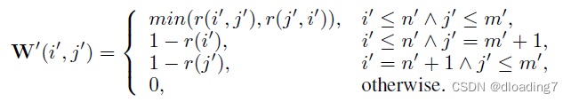
coarse-level的gt confidence matrix由以下方式生成（注意dustbin处的gt生成）：

coarse loss由SuperGlue-style sinkhorn生成的confidence matrix与以上gt confidence matrix计算得到，计算方式为加权交叉熵损失：

finer scale loss

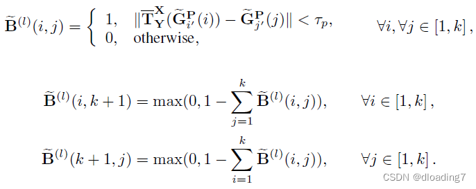
目的是监督point feature，finer-level的gt confidence matrix由以下方式生成（注意dustbin处的gt生成）：

finer loss由RPMNet-style sinkhorn生成的confidence matrix与以上gt confidence matrix计算得到，同样计算方式为加权交叉熵损失：

最终total loss为两者之和：$L=L_c+\lambda L_f$.

Experiments

由于CoFiNet是detection-free的模型，首先生成coarse-correspondences，接着refine成point-correspondences，因此与之前的配准工作不同，在测试阶段不存在对src与tgt进行固定点数采样再进行配准的说法，因此为了在测试阶段与先前的工作保持一致，CoFiNet中的“固定点数采样”定义为对最终生成的point-correspondences进行采样，即“采样5000点”等价于在CoFiNet中采样5000对point-correspondences，采样使用概率采样probablistically sampling，每对correspondences被采样到的概率正比于:
$$c_{global}=c_{fine}\cdot c_{coarse}$$

其中$c_{coarse}$与$c_{fine}$分别代表coarse-level与finer-level阶段得到的node confidence与point confidence.

模型默认训练150epochs，时间太久，这里选择使用训练了30个epoch的保存模型model_best_matching_recall.pth进行测试，
实验结果如下（open3d 0.9.0）：

Dataset -> 3DMatch	5000	2500	1000	500	250
metric	IR	IR	IR	IR	IR
PREDATOR (paper)	58.0	58.4	57.1	54.1	49.3
CoFiNet (paper)	49.8	51.2	51.9	52.2	52.2
pretrained weights	49.9	51.2	52.0	52.3	52.1
model_best_matching_recall.pth (30 epochs)	50.0	51.0	51.5	51.7	51.8
metric	FMR	FMR	FMR	FMR	FMR
PREDATOR (paper)	96.6	96.6	96.5	96.3	96.5
CoFiNet (paper)	98.1	98.3	98.1	98.2	98.3
pretrained weights	98.1	98.3	98.0	98.3	98.3
model_best_matching_recall.pth (30 epochs)	97.6	97.4	97.4	97.8	97.3
metric	RR	RR	RR	RR	RR
PREDATOR (paper)	89.0	89.9	90.6	88.5	86.6
CoFiNet (paper)	89.3	88.9	88.4	87.4	87.0
pretrained weights	88.0	87.6	87.4	86.7	85.1
model_best_matching_recall.pth (30 epochs)	87.4	87.1	87.6	85.6	86.4

Dataset -> 3DLoMatch	5000	2500	1000	500	250
metric	IR	IR	IR	IR	IR
PREDATOR (paper)	26.7	28.1	28.3	27.5	25.8
CoFiNet (paper)	24.4	25.9	26.7	26.8	26.9
pretrained weights	24.4	25.8	26.7	26.9	27.0
model_best_matching_recall.pth (30 epochs)	24.8	25.8	26.5	26.6	26.9
metric	FMR	FMR	FMR	FMR	FMR
PREDATOR (paper)	78.6	77.4	76.3	75.7	75.3
CoFiNet (paper)	83.1	83.5	83.3	83.1	82.6
pretrained weights	83.1	83.0	82.9	82.8	82.4
model_best_matching_recall.pth (30 epochs)	81.4	82.0	82.2	81.5	82.3
metric	RR	RR	RR	RR	RR
PREDATOR (paper)	59.8	61.2	62.4	60.8	58.1
CoFiNet (paper)	67.5	66.2	64.2	63.1	61.0
pretrained weights	62.3	62.6	62.0	60.9	58.1
model_best_matching_recall.pth (30 epochs)	60.2	60.5	59.8	59.5	57.0

Conclusion

• 根据以上表格结果，CoFiNet的复现结果除了在3DLoMatch benchmark上的RR结果相较于文章中较低以外，其余部分大致能与文章中给出数字保持一致；
• CoFiNet是点云配准中第一个使用coarse-to-fine思想的工作，对以后的工作具有不小的启发意义，最直接的就是CVPR2022中的另一个工作GeoFormer[10]，同样是基于以上思想；
• 基于Sinkhorn迭代方式生成correspondences的方式相比于普通的feature-matching方式确实更为优雅。

PS

在代码实现中，发现有两个点比较有意思，第一是coarse-level的gt confidence matrix的生成方式并不是完全与文章中给出的方式一致，即：

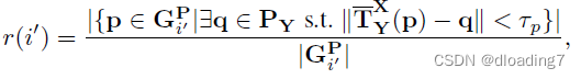
而实际代码中，对于$r\left(i^{\prime },j^{\prime }\right)$的计算与论文中给出的式（4）还是存在一些出入，从具体代码中可知，$r\left(i^{\prime },j^{\prime }\right)$的实际计算方式为：
$$r\left(i^{\prime },j^{\prime }\right)=\frac{\left|\left\{p\in G_{i^{\prime }}^P,q\in G_{j^{\prime }}^P|s.t.\Vert {\bar{T}}_Y^X\left(p\right)-q\Vert \le {\tau }_p\right\}\right|}{\left|\left\{p\in G_{i^{\prime }}^P,q\in P_Y|s.t.\Vert {\bar{T}}_Y^X\left(p\right)-q\Vert \le {\tau }_p\right\}\right|}$$
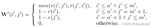
并且对于以上gt confidence matrix $W^{\prime }\left(i^{\prime },j^{\prime }\right)$的$i^{\prime }\le n^{\prime }\wedge j^{\prime }\le m^{\prime }$处，$W^{\prime }\left(i^{\prime },j^{\prime }\right)$的实际取值方式为：
$$\min \left(r\left(i^{\prime },j^{\prime }\right)\ast r\left(i^{\prime }\right),r\left(j^{\prime },i^{\prime }\right)\ast r\left(j^{\prime }\right)\right)$$

第二点是关于sinkhorn代码的实现，整体模型一共有两处需要使用sinkhorn迭代，一处是corase-scale的correspondences proposal处，一处是density-adaptive matching处，那么观察CoFiNet的代码可以发现，在以上两处作者选择了两种sinkhorn的实现方式，前者使用的是SuperGlue式sinkhorn，后者使用的是RPMNet式sinkhorn，两种实现方式其实是有一些差别的，具体为何在两处使用不同方式的sinkhorn迭代实现，目前尚且没有找到原因，可能得等作者自己在issue中回应。

References

[1] Yu H, Li F, Saleh M, et al. Cofinet: Reliable coarse-to-fine correspondences for robust pointcloud registration[J]. Advances in Neural Information Processing Systems, 2021, 34: 23872-23884.
[2] Sun J, Shen Z, Wang Y, et al. LoFTR: Detector-free local feature matching with transformers[C]//Proceedings of the IEEE/CVF conference on computer vision and pattern recognition. 2021: 8922-8931.
[3] Thomas H, Qi C R, Deschaud J E, et al. Kpconv: Flexible and deformable convolution for point clouds[C]//Proceedings of the IEEE/CVF international conference on computer vision. 2019: 6411-6420.
[4] Bai X, Luo Z, Zhou L, et al. D3feat: Joint learning of dense detection and description of 3d local features[C]//Proceedings of the IEEE/CVF conference on computer vision and pattern recognition. 2020: 6359-6367.
[5] Huang S, Gojcic Z, Usvyatsov M, et al. Predator: Registration of 3d point clouds with low overlap[C]//Proceedings of the IEEE/CVF Conference on computer vision and pattern recognition. 2021: 4267-4276.
[6] Li Y, Harada T. Lepard: Learning partial point cloud matching in rigid and deformable scenes[C]//Proceedings of the IEEE/CVF Conference on Computer Vision and Pattern Recognition. 2022: 5554-5564.
[7] Zhu L, Guan H, Lin C, et al. Neighborhood-aware Geometric Encoding Network for Point Cloud Registration[J]. arXiv preprint arXiv:2201.12094, 2022.
[8] Sarlin P E, DeTone D, Malisiewicz T, et al. Superglue: Learning feature matching with graph neural networks[C]//Proceedings of the IEEE/CVF conference on computer vision and pattern recognition. 2020: 4938-4947.
[9] Yew Z J, Lee G H. Rpm-net: Robust point matching using learned features[C]//Proceedings of the IEEE/CVF conference on computer vision and pattern recognition. 2020: 11824-11833.
[10] Qin Z, Yu H, Wang C, et al. Geometric transformer for fast and robust point cloud registration[C]//Proceedings of the IEEE/CVF Conference on Computer Vision and Pattern Recognition. 2022: 11143-11152.