昇思25天学习打卡营第23天|K近邻算法实现红酒聚类

109702008

于 2024-07-11 12:18:33 发布

阅读量419

点赞数 2

分类专栏：人工智能 # python 文章标签：近邻算法聚类机器学习

本文链接：https://blog.csdn.net/eidolon_foot/article/details/140123571

版权

人工智能同时被 2 个专栏收录

212 篇文章 2 订阅

订阅专栏

python

130 篇文章 0 订阅

订阅专栏

学AI还能赢奖品？每天30分钟，25天打通AI任督二脉 (qq.com)

K近邻算法实现红酒聚类

本实验主要介绍使用MindSpore在部分wine数据集上进行KNN实验。

1、实验目的

了解KNN的基本概念；
了解如何使用MindSpore进行KNN实验。

2、K近邻算法原理介绍

K近邻算法（K-Nearest-Neighbor, KNN）是一种用于分类和回归的非参数统计方法，最初由 Cover和Hart于1968年提出(Cover等人,1967)，是机器学习最基础的算法之一。它正是基于以上思想：要确定一个样本的类别，可以计算它与所有训练样本的距离，然后找出和该样本最接近的k个样本，统计出这些样本的类别并进行投票，票数最多的那个类就是分类的结果。KNN的三个基本要素：

K值，一个样本的分类是由K个邻居的“多数表决”确定的。K值越小，容易受噪声影响，反之，会使类别之间的界限变得模糊。
距离度量，反映了特征空间中两个样本间的相似度，距离越小，越相似。常用的有Lp距离（p=2时，即为欧式距离）、曼哈顿距离、海明距离等。
分类决策规则，通常是多数表决，或者基于距离加权的多数表决（权值与距离成反比）。

非参数统计方法是指不依赖于参数化形式（如传统统计中的正态分布假设等）的统计方法，即它们对数据分布没有严格的假设。相对于参数统计方法（如线性回归、t检验等），非参数统计方法更为灵活，因为它们不假设数据遵循特定的分布模式。

参数统计方法依赖于对数据分布做出特定的假设和要求，并通过某些参数来描述数据的分布形态。这些参数化形式可以显著简化模型和分析，但也需要这些假设和参数与实际数据相符合，当假设不满足时，可能会导致误导性的结论。
1. 线性回归（Linear Regression）：
假设：因变量（响应变量）与自变量（解释变量）之间存在线性关系。
参数：回归系数（斜率和截距），通常假设误差项具有零均值、常方差（同方差性）和正态分布。
2. Logistic回归（Logistic Regression）：
假设：因变量（分类变量）满足逻辑斯蒂回归模型，回归系数是固定值。
参数：回归系数，用于描述自变量对因变量的影响，通过最大似然估计进行估计。
3. t检验（t-test）：
假设：样本数据来自于正态分布的总体。
参数：均值和方差，单样本t检验假设总体均值，双样本t检验假设两个总体的均值之间的差异。

2.1 分类问题

预测算法（分类）的流程如下：

（1）在训练样本集中找出距离待测样本x_test最近的k个样本，并保存至集合N中；

（2）统计集合N中每一类样本的个数𝐶𝑖,𝑖=1,2,3,...,𝑐；

（3）最终的分类结果为argmax𝐶𝑖 （最大的对应的𝐶𝑖）那个类。

在上述实现过程中，k的取值尤为重要。它可以根据问题和数据特点来确定。在具体实现时，可以考虑样本的权重，即每个样本有不同的投票权重，这种方法称为带权重的k近邻算法，它是一种变种的k近邻算法。

2.2 回归问题

假设离测试样本最近的k个训练样本的标签值为𝑦𝑖，则对样本的回归预测输出值为：

即为所有邻居的标签均值。

带样本权重的回归预测函数为：

其中𝑤𝑖为第个𝑖样本的权重。

2.3 距离的定义

KNN算法的实现依赖于样本之间的距离，其中最常用的距离函数就是欧氏距离（欧几里得距离）。ℝ𝑛空间中的两点𝑥和𝑦，它们之间的欧氏距离定义为：

需要特别注意的是，使用欧氏距离时，应将特征向量的每个分量归一化，以减少因为特征值的尺度范围不同所带来的干扰，否则数值小的特征分量会被数值大的特征分量淹没。

其它的距离计算方式还有Mahalanobis距离、Bhattacharyya距离等。

3、实验环境

预备知识：

熟练使用Python。
具备一定的机器学习理论知识，如KNN、无监督学习、欧式距离等。

实验环境：

MindSpore 2.0（MindSpore版本会定期更新，本指导也会定期刷新，与版本配套）；
本案例支持win_x86和Linux系统，CPU/GPU/Ascend均可运行。
如果在本地运行此实验，请参考《MindSpore环境搭建实验手册》在本地安装MindSpore。

4、数据处理

4.1 数据准备

Wine数据集是模式识别最著名的数据集之一，Wine数据集的官网：Wine Data Set。这些数据是对来自意大利同一地区但来自三个不同品种的葡萄酒进行化学分析的结果。数据集分析了三种葡萄酒中每种所含13种成分的量。这些13种属性是

Alcohol，酒精
Malic acid，苹果酸
Ash，灰
Alcalinity of ash，灰的碱度
Magnesium，镁
Total phenols，总酚
Flavanoids，类黄酮
Nonflavanoid phenols，非黄酮酚
Proanthocyanins，原花青素
Color intensity，色彩强度
Hue，色调
OD280/OD315 of diluted wines，稀释酒的OD280/OD315
Proline，脯氨酸

方式一，从Wine数据集官网下载wine.data文件。
方式二，从华为云OBS中下载wine.data文件。

Key	Value	Key	Value
Data Set Characteristics:	Multivariate	Number of Instances:	178
Attribute Characteristics:	Integer, Real	Number of Attributes:	13
Associated Tasks:	Classification	Missing Values?	No

%%capture captured_output
# 实验环境已经预装了mindspore==2.2.14，如需更换mindspore版本，可更改下面mindspore的版本号
!pip uninstall mindspore -y
!pip install -i https://pypi.mirrors.ustc.edu.cn/simple mindspore==2.2.14

# 查看当前 mindspore 版本
!pip show mindspore

Name: mindspore
Version: 2.2.14
Summary: MindSpore is a new open source deep learning training/inference framework that could be used for mobile, edge and cloud scenarios.
Home-page: https://www.mindspore.cn
Author: The MindSpore Authors
Author-email: contact@mindspore.cn
License: Apache 2.0
Location: /home/nginx/miniconda/envs/jupyter/lib/python3.9/site-packages
Requires: asttokens, astunparse, numpy, packaging, pillow, protobuf, psutil, scipy
Required-by:

from download import download

# 下载红酒数据集
url = "https://ascend-professional-construction-dataset.obs.cn-north-4.myhuaweicloud.com:443/MachineLearning/wine.zip"  
path = download(url, "./", kind="zip", replace=True)

Downloading data from https://ascend-professional-construction-dataset.obs.cn-north-4.myhuaweicloud.com:443/MachineLearning/wine.zip (4 kB)

file_sizes: 100%|██████████████████████████| 4.09k/4.09k [00:00<00:00, 2.51MB/s]
Extracting zip file...
Successfully downloaded / unzipped to ./

4.2 数据读取与处理

导入MindSpore模块和辅助模块

在生成数据之前，导入需要的Python库。

目前使用到os库，为方便理解，其他需要的库，我们在具体使用到时再说明。

详细的MindSpore的模块说明，可以在MindSpore API页面中搜索查询。

可以通过context.set_context来配置运行需要的信息，譬如运行模式、后端信息、硬件等信息。

导入context模块，配置运行需要的信息。

%matplotlib inline
import os
import csv
import numpy as np
import matplotlib.pyplot as plt

import mindspore as ms
from mindspore import nn, ops

ms.set_context(device_target="CPU")

参考mindspore.set_context ，device_target (str) - 表示待运行的目标设备，支持 ‘Ascend’、 ‘GPU’和 ‘CPU’。如果未设置此参数，则使用MindSpore包对应的后端设备。这里在实验环境中还可以设置为Ascend。

读取Wine数据集`wine.data`，并查看部分数据。

with open('wine.data') as csv_file:
    data = list(csv.reader(csv_file, delimiter=','))
print(data[56:62]+data[130:133])

[['1', '14.22', '1.7', '2.3', '16.3', '118', '3.2', '3', '.26', '2.03', '6.38', '.94', '3.31', '970'], ['1', '13.29', '1.97', '2.68', '16.8', '102', '3', '3.23', '.31', '1.66', '6', '1.07', '2.84', '1270'], ['1', '13.72', '1.43', '2.5', '16.7', '108', '3.4', '3.67', '.19', '2.04', '6.8', '.89', '2.87', '1285'], ['2', '12.37', '.94', '1.36', '10.6', '88', '1.98', '.57', '.28', '.42', '1.95', '1.05', '1.82', '520'], ['2', '12.33', '1.1', '2.28', '16', '101', '2.05', '1.09', '.63', '.41', '3.27', '1.25', '1.67', '680'], ['2', '12.64', '1.36', '2.02', '16.8', '100', '2.02', '1.41', '.53', '.62', '5.75', '.98', '1.59', '450'], ['3', '12.86', '1.35', '2.32', '18', '122', '1.51', '1.25', '.21', '.94', '4.1', '.76', '1.29', '630'], ['3', '12.88', '2.99', '2.4', '20', '104', '1.3', '1.22', '.24', '.83', '5.4', '.74', '1.42', '530'], ['3', '12.81', '2.31', '2.4', '24', '98', '1.15', '1.09', '.27', '.83', '5.7', '.66', '1.36', '560']]

取三类样本（共178条），将数据集的13个属性作为自变量𝑋。将数据集的3个类别作为因变量𝑌。¶

X = np.array([[float(x) for x in s[1:]] for s in data[:178]], np.float32)
Y = np.array([s[0] for s in data[:178]], np.int32)

取样本的某两个属性进行2维可视化，可以看到在某两个属性上样本的分布情况以及可分性。

attrs = ['Alcohol', 'Malic acid', 'Ash', 'Alcalinity of ash', 'Magnesium', 'Total phenols',
         'Flavanoids', 'Nonflavanoid phenols', 'Proanthocyanins', 'Color intensity', 'Hue',
         'OD280/OD315 of diluted wines', 'Proline']
plt.figure(figsize=(10, 8))
for i in range(0, 4):
    plt.subplot(2, 2, i+1)
    a1, a2 = 2 * i, 2 * i + 1
    plt.scatter(X[:59, a1], X[:59, a2], label='1')
    plt.scatter(X[59:130, a1], X[59:130, a2], label='2')
    plt.scatter(X[130:, a1], X[130:, a2], label='3')
    plt.xlabel(attrs[a1])
    plt.ylabel(attrs[a2])
    plt.legend()
plt.show()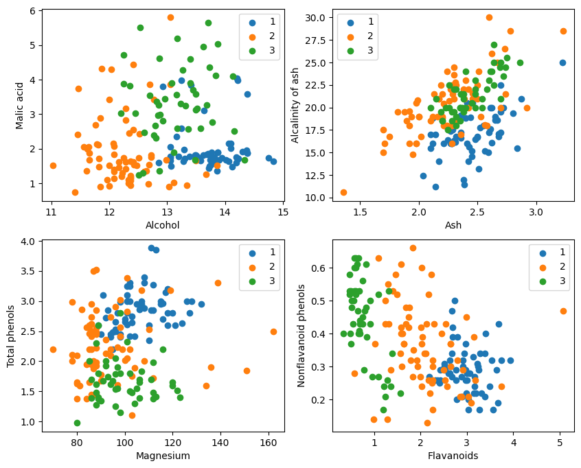

从代码估计可能前59个样本是1类，59~130是2类，剩余的是3类。

从图形显示看，左上角和右下角的图形中的两个属性分类效果比较好，特别是1、2类界限比较明显。

将数据集按128:50划分为训练集（已知类别样本）和验证集（待验证样本）：¶

train_idx = np.random.choice(178, 128, replace=False)
test_idx = np.array(list(set(range(178)) - set(train_idx)))
X_train, Y_train = X[train_idx], Y[train_idx]
X_test, Y_test = X[test_idx], Y[test_idx]

分解test_idx = np.array(list(set(range(178)) - set(train_idx)))
1. range(178) 生成从 0 到 177 的整数序列。
2. set(range(178)) 将这个整数序列转换为集合。集合是一种不允许重复元素的数据结构，支持高效的集合运算（如并、交、差集等）。
3. set(train_idx) 将随机选择的训练集索引列表 train_idx 转换为集合。
4. set(range(178)) - set(train_idx) 计算集合的差集运算，得到那些在 set(range(178)) 但不在 set(train_idx) 中的元素，也就是测试集的索引。这是一个集合运算，能够快速、高效地计算出差异元素。
5. list(...) 将差集运算的结果转换回列表。
6. np.array(...) 将这个列表转换为 numpy 数组，以便与 numpy 数组 X 和 Y 进行索引操作。

5、模型构建--计算距离

利用MindSpore提供的tile, square, ReduceSum, sqrt, TopK等算子，通过矩阵运算的方式同时计算输入样本x和已明确分类的其他样本X_train的距离，并计算出top k近邻

class KnnNet(nn.Cell):
    def __init__(self, k):
        super(KnnNet, self).__init__()
        self.k = k

    def construct(self, x, X_train):
        #平铺输入x以匹配X_train中的样本数
        x_tile = ops.tile(x, (128, 1))
        square_diff = ops.square(x_tile - X_train)
        square_dist = ops.sum(square_diff, 1)
        dist = ops.sqrt(square_dist)
        #-dist表示值越大，样本就越接近
        values, indices = ops.topk(-dist, self.k)
        return indices

def knn(knn_net, x, X_train, Y_train):
    x, X_train = ms.Tensor(x), ms.Tensor(X_train)
    indices = knn_net(x, X_train)
    topk_cls = [0]*len(indices.asnumpy())
    for idx in indices.asnumpy():
        topk_cls[Y_train[idx]] += 1
    cls = np.argmax(topk_cls)
    return cls

1. 定义KNN网络类：KnnNet
__init__函数：初始化网络，设置K值（即选取的最近邻数量）。
construct函数：计算输入样本 x 与训练集 X_train 中每一个样本之间的欧氏距离，并返回距离最小的k个（即最近邻）样本的索引。
2. 定义KNN函数：knn
接收knn_net（KNN网络实例），测试样本x，训练样本X_train和训练标签Y_train作为输入。
使用knn_net找到x的k个最近邻样本，并依据这些样本的标签进行分类，返回分类结果（即预测的类别）。

6、模型预测

在验证集上验证KNN算法的有效性，取𝑘=5，验证精度接近80%，说明KNN算法在该3分类任务上有效，能根据酒的13种属性判断出酒的品种。

acc = 0
knn_net = KnnNet(5)
for x, y in zip(X_test, Y_test):
    pred = knn(knn_net, x, X_train, Y_train)
    acc += (pred == y)
    print('label: %d, prediction: %s' % (y, pred))
print('Validation accuracy is %f' % (acc/len(Y_test)))

计算并打印测试集的准确率
循环遍历测试集 X_test 和 Y_test 中的每一个样本，利用 knn 函数对每个样本进行分类。
统计预测正确的样本数量，计算并输出分类的准确率。

label: 1, prediction: 1
label: 2, prediction: 3
label: 1, prediction: 1
label: 1, prediction: 1
label: 3, prediction: 2
label: 1, prediction: 1
label: 1, prediction: 1
label: 3, prediction: 3
label: 1, prediction: 1
label: 1, prediction: 1
label: 1, prediction: 1
label: 1, prediction: 1
label: 3, prediction: 2
label: 1, prediction: 2
label: 1, prediction: 1
label: 1, prediction: 1
label: 3, prediction: 2
label: 1, prediction: 1
label: 1, prediction: 1
label: 3, prediction: 3
label: 3, prediction: 1
label: 3, prediction: 2
label: 3, prediction: 2
label: 1, prediction: 1
label: 1, prediction: 1
label: 3, prediction: 2
label: 1, prediction: 3
label: 3, prediction: 1
label: 3, prediction: 3
label: 3, prediction: 1
label: 3, prediction: 1
label: 1, prediction: 1
label: 1, prediction: 1
label: 1, prediction: 1
label: 1, prediction: 1
label: 2, prediction: 2
label: 2, prediction: 2
label: 2, prediction: 3
label: 2, prediction: 3
label: 2, prediction: 2
label: 2, prediction: 2
label: 2, prediction: 2
label: 2, prediction: 1
label: 2, prediction: 3
label: 2, prediction: 2
label: 2, prediction: 2
label: 2, prediction: 2
label: 2, prediction: 2
label: 2, prediction: 2
label: 2, prediction: 2
Validation accuracy is 0.660000

不是每次都能达到80%，试了多次，终于有一次精确度到了80%：

label: 1, prediction: 1
label: 3, prediction: 3
label: 1, prediction: 1
label: 1, prediction: 1
label: 3, prediction: 3
label: 3, prediction: 3
label: 3, prediction: 2
label: 3, prediction: 3
label: 1, prediction: 1
label: 3, prediction: 3
label: 1, prediction: 1
label: 1, prediction: 3
label: 3, prediction: 3
label: 1, prediction: 3
label: 1, prediction: 1
label: 3, prediction: 3
label: 1, prediction: 1
label: 1, prediction: 1
label: 3, prediction: 3
label: 3, prediction: 3
label: 3, prediction: 2
label: 1, prediction: 1
label: 3, prediction: 3
label: 1, prediction: 1
label: 3, prediction: 3
label: 1, prediction: 1
label: 1, prediction: 1
label: 1, prediction: 1
label: 1, prediction: 1
label: 1, prediction: 1
label: 1, prediction: 1
label: 1, prediction: 1
label: 2, prediction: 3
label: 2, prediction: 1
label: 2, prediction: 2
label: 2, prediction: 2
label: 2, prediction: 2
label: 2, prediction: 2
label: 2, prediction: 3
label: 2, prediction: 2
label: 2, prediction: 2
label: 2, prediction: 2
label: 2, prediction: 3
label: 2, prediction: 2
label: 2, prediction: 2
label: 2, prediction: 2
label: 2, prediction: 2
label: 2, prediction: 2
label: 2, prediction: 3
label: 2, prediction: 2
Validation accuracy is 0.820000

实验小结

本实验使用MindSpore实现了KNN算法，用来解决3分类问题。取wine数据集上的3类样本，分为已知类别样本和待验证样本，从验证结果可以看出KNN算法在该任务上有效，能根据酒的13种属性判断出酒的品种。

数据准备：从Wine数据集官网或华为云OBS下载数据，进行读取和处理。

数据处理：将数据集分为自变量（13种属性）和因变量（3个类别），进行可视化以观察样本分布。

模型构建：定义KNN网络结构，利用MindSpore提供的算子计算输入样本与训练样本之间的距离，找出最近的k个邻居。

模型预测：在验证集上进行预测，计算预测准确率。

实验结果显示，KNN算法在Wine数据集上的分类准确率接近80%（66%）。

109702008

关注

2
点赞
踩
6

收藏

觉得还不错? 一键收藏
打赏
0
评论
昇思25天学习打卡营第23天|K近邻算法实现红酒聚类

K近邻算法（K-Nearest-Neighbor, KNN）是一种用于分类和回归的非参数统计方法，最初由 Cover和Hart于1968年提出(Cover等人,1967)，是机器学习最基础的算法之一。它正是基于以上思想：要确定一个样本的类别，可以计算它与所有训练样本的距离，然后找出和该样本最接近的k个样本，统计出这些样本的类别并进行投票，票数最多的那个类就是分类的结果。KNN的三个基本要素：K值，一个样本的分类是由K个邻居的“多数表决”确定的。K值越小，容易受噪声影响，反之，会使类别之间的界限变得模糊。
复制链接

扫一扫