Piecewise Jerk Path Optimizer的python实现 ce758b3840a84d069264848dfb88dde6

最新推荐文章于 2024-05-03 20:05:36 发布

datou_zjq

最新推荐文章于 2024-05-03 20:05:36 发布

阅读量1k

点赞数

分类专栏：规划控制自动驾驶文章标签：算法自动驾驶

本文链接：https://blog.csdn.net/fengdehuhuan122/article/details/120191590

版权

规划控制同时被 2 个专栏收录

1 篇文章 0 订阅

订阅专栏

自动驾驶

1 篇文章 0 订阅

订阅专栏

Piecewise Jerk Path Optimizer的python实现

Piecewise Jerk Path Optimizer的相关知识点可参考文末的两篇文章，本文主要是进行该算法的问题构造和实现。

cost function

$J=w_x\sum^{n-1}_{i=0}(x_i-r_i)^2+w_{x'}\sum^{n-1}_{i=0}(x'_i)^2+w_{x''}\sum^{n-1}_{i=0}(x''_i)^2+w_{x'''}\sum^{n-2}_{i=0}(x'''_i)^2$

qp problem

$min\{\frac{1}{2}x^TPx+qx\}\\l\le Ax\le u$

本文使用osqp进行二次规划问题的求解。

构造P和q矩阵

由 $x'''_i\Delta s=x''_{i+1}-x''_i$ ，得到 $x'''_i=\frac{x''_{i+1}-x''_i}{\Delta s}$ ，将其带入J中，可得

$J=w_x\sum^{n-1}_{i=0}[(x_i)^2+(r_i)^2-2x_ir_i]+w_{x'}\sum^{n-1}_{i=0}(x'_i)^2+w_{x''}\sum^{n-1}_{i=0}(x''_i)^2+\frac{w_{x'''}}{\Delta s^2}\sum^{n-2}_{i=0}[(x''_{i+1})^2+(x''_i)^2-2x''_{i+1}x''_i]$

整理可得（去掉常数项）：

$J=w_x\sum^{n-1}_{i=0}[(x_i)^2-2x_ir_i]+w_{x'}\sum^{n-1}_{i=0}(x'_i)^2+(w_{x''}+\frac{2w_{x'''}}{\Delta s^2})\sum^{n-1}_{i=0}(x''_i)^2-\frac{w_{x'''}}{\Delta s^2}(x''_0+x''_{n-1})-\frac{2w_{x'''}}{\Delta s^2}\sum^{n-2}_{i=0}(x''_{i+1}x''_i)$

令：

$x=\begin{bmatrix} x_0 \\[4pt] x_1\\[4pt]\vdots \\[4pt]x_{n-1}\\[4pt]x'_0\\[4pt]x'_1\\[4pt]\vdots\\[4pt]x'_{n-1}\\[4pt]x''_0\\[4pt]x''_1\\[4pt]\vdots\\[4pt]x''_{n-1} \end{bmatrix}\in R^{3n \times 1}$

则：

$P_x=\begin{bmatrix} w_x &0& \ldots&0\\0&w_x&\ldots&0\\\vdots&\vdots&\ddots&\vdots\\0&0&\ldots&w_x \end{bmatrix}\in R^{n \times n}$

$P_{x'}=\begin{bmatrix} w_{x'} &0& \ldots&0\\0&w_{x'}&\ldots&0\\\vdots&\vdots&\ddots&\vdots\\0&0&\ldots&w_{x'} \end{bmatrix}\in R^{n \times n}$

$P_{x''}=\begin{bmatrix} w_{x''}+\frac{w_{x'''}}{\Delta s^2} &0& \ldots&0&0\\[8pt]-\frac{2w_{x'''}}{\Delta s^2}&w_{x''}+\frac{2w_{x'''}}{\Delta s^2}&\ldots&0&0\\[8pt]\vdots&\vdots&\ddots&\vdots&\vdots\\[8pt]0&0&\ldots&w_{x''}+\frac{2w_{x'''}}{\Delta s^2}&0\\[8pt]0&0&\ldots&-\frac{2w_{x'''}}{\Delta s^2}&w_{x''}+\frac{w_{x'''}}{\Delta s^2} \end{bmatrix}\in R^{n \times n}$

$P=\begin{bmatrix} P_x &0&0\\0&P_{x'}&0\\0&0&P_{x''} \end{bmatrix}\in R^{3n \times 3n}$

$q=\begin{bmatrix} -r_0\\-r_1\\\vdots\\-r_{n-1}\\0\\\vdots\\0 \end{bmatrix}^T\in R^{1 \times 3n}$

构造不等式矩阵

$x_{i+1}=x_i+x'_i\Delta s+\frac{1}{2}\Delta s^2x''_i+\frac{1}{6}\Delta s^3x'''_i$

$x'_{i+1}=x'_i+x''_i\Delta s+\frac{1}{2}\Delta s^2x'''_i$

将 $x'''_i$ 提取出来，可以得到：

$x'''_i\frac{\Delta s^3}{6}=x_{i+1}-x_i-x'_i\Delta s-\frac{1}{2}\Delta s^2x''_i$

$x'''_i\frac{\Delta s^2}{2}=x'_{i+1}-x'_i-x''_i\Delta s$

令

$A_x=I \in R^{3n\times3n}$

$A_{ds}=-\Delta sI \in R^{n\times n}$

$A_{ds^2}=-\frac{1}{2}\Delta s^2I \in R^{n\times n}$

$A_{I}=\begin{bmatrix} -1 &1& 0&\ldots&0 \\0&-1&1&\ldots&0 \\\vdots&\vdots&\ddots&\ddots&\vdots \\0&0&\ldots&-1&1 \\0&0&\ldots&0&-1 \end{bmatrix}\in R^{n \times n}$

$A=\begin{bmatrix} &A_x\\A_I&A_{ds}&A_{ds^2} \\0&A_I&A_{ds} \end{bmatrix}\in R^{5n \times 3n}$

上下边界：

$l=\begin{bmatrix} x_{0l}\\[8pt]\vdots \\[8pt]x_{(n-1)l}\\[8pt]x'_{0l}\\[8pt]\vdots\\[8pt]x'_{(n-1)l}\\[8pt]x''_{0l}\\[8pt]\vdots\\[8pt]x''_{(n-1)l}\\[8pt]-\frac{\Delta s^3}{6}x'''_{bound}\\[8pt]\vdots\\[8pt]-\frac{\Delta s^3}{6}x'''_{bound}\\[8pt]-\frac{\Delta s^2}{2}x'''_{bound}\\[8pt]\vdots\\[8pt]-\frac{\Delta s^2}{2}x'''_{bound} \end{bmatrix}\in R^{5n \times 1}$

$u=\begin{bmatrix} x_{0u}\\[8pt]\vdots \\[8pt]x_{(n-1)u}\\[8pt]x'_{0u}\\[8pt]\vdots\\[8pt]x'_{(n-1)u}\\[8pt]x''_{0u}\\[8pt]\vdots\\[8pt]x''_{(n-1)u}\\[8pt]\frac{\Delta s^3}{6}x'''_{bound}\\[8pt]\vdots\\[8pt]\frac{\Delta s^3}{6}x'''_{bound}\\[8pt]\frac{\Delta s^2}{2}x'''_{bound}\\[8pt]\vdots\\[8pt]\frac{\Delta s^2}{2}x'''_{bound} \end{bmatrix}\in R^{5n \times 1}$

构造好矩阵后，使用Python实现

import matplotlib.pyplot as plt
import osqp
import numpy as np
from scipy import sparse
import random
# 障碍物设置
obs = [[5,10,2,3],[15,20,-2,-0.5],[25,30,0,1]]#start_s,end_s,l_low,l_up

s_len = 50
delta_s = 0.1
n = int(s_len / delta_s)
x = np.linspace(0,s_len,n)
up_bound = [0]*(5*n + 3)
low_bound = [0]*(5*n + 3)
s_ref = [0]*3*n

dddl_bound = 0.01

####################边界提取################
l_bound = 5
for i in range(n):
    for j in range(len(obs)):
        if x[i] >= obs[j][0] and x[i] <= obs[j][1]:            
            low_ = obs[j][2]
            up_ = obs[j][3]         
            break
        else:
            up_ = l_bound
            low_ = -l_bound
    up_bound[i] = up_
    low_bound[i] = low_   
    s_ref[i] = 0.5*(up_ + low_)

# cotinue_i = True
# for i in range(n):
#     x_tmp = x[i]
#     if cotinue_i:
#         i_start = i
#         up_ = random.randint(1, 3) * 0.1
#         low_ = random.randint(-3, -1) * 0.1
#         if up_ < low_:
#             tmp = up_
#             up_ = low_
#             low_ = tmp
#         cotinue_i = False
#     if i - i_start >= obs_len / delta_s:
#         cotinue_i = True
#     up_bound[i] = up_
#     low_bound[i] = low_
#     s_ref[i] = 0.5*(up_ + low_)
    
for i in range(3*n,4*n):
    up_bound[i] = dddl_bound * delta_s *delta_s *delta_s/6
    low_bound[i] = -dddl_bound * delta_s *delta_s *delta_s/6  
for i in range(4*n,5*n):
    up_bound[i] = dddl_bound * delta_s *delta_s / 2
    low_bound[i] = -dddl_bound * delta_s *delta_s / 2
    
    

####################构造P和Q################
w_l = 0.005
w_dl = 1
w_ddl = 1
w_dddl = 0.1
eye_n = np.identity(n)
zero_n = np.zeros((n, n))

P_zeros = zero_n
P_l = w_l * eye_n
P_dl = w_dl * eye_n
P_ddl = (w_ddl + 2*w_dddl/delta_s/delta_s) * eye_n -2 * w_dddl / delta_s/delta_s* np.eye(n,k = -1)
P_ddl[0][0] = w_ddl + w_dddl/delta_s/delta_s
P_ddl[n-1][n-1] = w_ddl + w_dddl/delta_s/delta_s

P = sparse.csc_matrix(np.block([
    [P_l,P_zeros,P_zeros],
    [P_zeros,P_dl,P_zeros],
    [P_zeros,P_zeros,P_ddl]
    ]))
q = np.array([-w_l*s_ for s_ in s_ref])

####################构造A和LU################

#构造：l(i+1) = l(i) + l'(i) * delta_s + 1/2 * l''(i) * delta_s^2 + 1/6 * l'''(i) * delta_s^3
A_ll = -eye_n + np.eye(n,k = 1)
A_ldl = -delta_s * eye_n
A_lddl = -0.5 * delta_s * delta_s * eye_n
A_l = (np.block([
    [A_ll,A_ldl,A_lddl]
    ]))

# 构造：l'(i+1) = l'(i) + l''(i) * delta_s + 1/2 * l'''(i) * delta_s^2
A_dll = zero_n
A_dldl = -eye_n + np.eye(n,k = 1)
A_dlddl =  -delta_s * eye_n
A_dl = np.block([
    [A_dll,A_dldl,A_dlddl]
    ])

A_ul = np.block([
    [eye_n,zero_n,zero_n],
    [zero_n,zero_n,zero_n],
    [zero_n,zero_n,zero_n]
    ])#3n*3n
# 初始化设置
A_init = np.zeros((3, 3*n))
A_init[0][0] = 1

A = sparse.csc_matrix(np.row_stack((A_ul,A_l,A_dl,A_init)))

low_bound[5*n] = 1
up_bound[5*n] = 1
l = np.array(low_bound)
u = np.array(up_bound)

# Create an OSQP object
prob = osqp.OSQP()

# Setup workspace and change alpha parameter
prob.setup(P, q, A, l, u, alpha=1.0)

# Solve problem
res = prob.solve()
    
plt.plot(u[:n],'.',color = 'blue')
plt.plot(l[:n],'.',color = 'black')
# plt.plot(s_ref[:n],'.')
plt.plot(res.x[:n],'.',color = 'red')
plt.show()

在这里插入图片描述

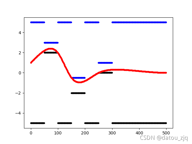
规划结果如上图所示，其中蓝色为上边界曲线，黑色为下边，红色为规划出的轨迹。

参考文章：

[1]https://zhuanlan.zhihu.com/p/325645742

[2]https://www.cnblogs.com/icathianrain/p/14407626.html

datou_zjq

关注

0
点赞
踩
2

收藏

觉得还不错? 一键收藏
0
评论
Piecewise Jerk Path Optimizer的python实现 ce758b3840a84d069264848dfb88dde6

Piecewise Jerk Path Optimizer的python实现Piecewise Jerk Path Optimizer的相关知识点可参考文末的两篇文章，本文主要是进行该算法的问题构造和实现。cost functionJ=wx∑i=0n−1(xi−ri)2+wx′∑i=0n−1(xi′)2+wx′′∑i=0n−1(xi′′)2+wx′′′∑i=0n−2(xi′′′)2J=w_x\sum^{n-1}_{i=0}(x_i-r_i)^2+w_{x'}\sum^{n-1}_{i=0}(x'_i)
复制链接

扫一扫