


本期内容

写在前面
今天分享一个关于KEGG通路图绘制的R包,也许在你后面的分析中可以使用得到。
在KEGG富集分析中,若我们要绘制某一个富集通路,一般回到KEGG官网中寻找该通路的富集图。然后,通过AI,PPT等等一系列手段进行绘制。但是,目前也有一些云平台可以使用,就看自己如何绘制。
今天,分享ggkegg包,一个用于绘制KEGG富集通路的R包,实用性也很强,以及作者提供了详细的帮助文档(PS:我们也基于机器翻译,整理了ggkegg的帮助文档,后面会提供给大家)。
2023教程汇总:2023年教程汇总 | 《小杜的生信笔记》
原文链接:ggkegg | 对KEGG数据进行可视化
加载R包
## 安装R包
BiocManager::install("ggkegg")
# or
devtools::install_github("noriakis/ggkegg")

##--------------------
library(ggkegg)
library(ggfx)
library(igraph)
library(tidygraph)
library(dplyr)
一个简单的例子01
pathway("ko01100") |>
    process_line() |>
    highlight_module(module("M00021")) |>
    highlight_module(module("M00338")) |>
    ggraph(x=x, y=y) +
        geom_node_point(size=1, aes(color=I(fgcolor),
            filter=fgcolor!="none" & type!="line")) +
        geom_edge_link0(width=0.1, aes(color=I(fgcolor),
            filter=type=="line"& fgcolor!="none")) +
        with_outer_glow(
            geom_edge_link0(width=1,
                aes(color=I(fgcolor),
                    filter=(M00021 | M00338))),
            colour="red", expand=5
        ) +
        with_outer_glow(
            geom_node_point(size=1.5,
                aes(color=I(fgcolor),
                    filter=(M00021 | M00338))),
            colour="red", expand=5
        ) +
        geom_node_text(size=2,
            aes(x=x, y=y,
                label=graphics_name,
                filter=name=="path:ko00270"),
            repel=TRUE, family="sans", bg.colour="white") +
        theme_void()

compounds <- c("cpd:C00100", "cpd:C00894", "cpd:C00894", "cpd:C05668",
    "cpd:C05668", "cpd:C01013", "cpd:C01013", "cpd:C00222",
    "cpd:C00222", "cpd:C00024")
g <- pathway("ko00640") |> mutate(mod=highlight_set_nodes(compounds, how="all"))
ggraph(g, layout="manual", x=x, y=y)+
    geom_node_rect(fill="grey",aes(filter=type == "ortholog"))+
    overlay_raw_map("ko00640")+
    geom_node_point(aes(filter=type == "compound"),
        shape=21, fill="blue", color="black", size=2)+
    ggfx::with_outer_glow(
        geom_node_point(aes(filter=mod, x=x, y=y), color="red",size=2),
        colour="yellow",expand=5
    )+
    theme_void()

g <- pathway("hsa04110")
pseudo_lfc <- sample(seq(0,3,0.1), length(V(g)), replace=TRUE)
names(pseudo_lfc) <- V(g)$name

ggkegg("hsa04110",
    convert_org = c("pathway","hsa","ko"),
    numeric_attribute = pseudo_lfc)+
    geom_edge_parallel2(
        aes(color=subtype_name),
        arrow = arrow(length = unit(1, 'mm')),
        start_cap = square(1, 'cm'),
        end_cap = square(1.5, 'cm')) +
    geom_node_rect(aes(filter=.data$type == "group"),
        fill="transparent", color="red") +
    geom_node_rect(aes(fill=numeric_attribute,
        filter=.data$type == "gene")) +
    geom_node_text(aes(label=converted_name,
        filter=.data$type == "gene"),
        size=2.5,
        color="black") +
    with_outer_glow(
        geom_node_text(aes(label=converted_name,
            filter=converted_name=="PCNA"),
            size=2.5, color="red"),
        colour="white", expand=4
    ) +
    scale_edge_color_manual(values=viridis::plasma(11)) +
    scale_fill_viridis(name="LFC") +
    theme_void()

常用例子02
多个微生物基因组评估模块完整性
跨多个微生物基因组评估模块完整性
mod <- module("M00009")
query <- sample(attr(mod, "definition_components"), 5) |>
  strsplit(":") |>
  sapply("[",2)
query
#> [1] "K01677" "K00164" "K00247" "K00240" "K00246"
mod |>
  module_completeness(query) |>
  kableExtra::kable()
我们可以评估从多个物种基因组中推断出的 KO 的完整性。在这里,我们将从 PATRIC 服务器获得的 MIDAS 流水线注释文件中可用的 EC 编号映射到 KO,并计算随机获得的物种的完整性。
## Load pre-computed KOs, and recursively perform completeness calculation.
mf <- list.files("../")
mf <- mf[startsWith(mf, "M")]
annos <- list()

candspid <- list.files("../species_dir")
candspid <- sample(candspid, 10)

## Obtain EC to KO mapping file from KEGG REST API
mapper <- data.table::fread("https://rest.kegg.jp/link/ec/ko", header=FALSE)

suppressMessages(
  for (i in candspid) {
    mcs <- NULL
    df <- read.table(paste0("../species_dir/",i), sep="\t", header=1)
    fid <- paste0("ec:",df[df$ontology=="ec",]$function_id)
    kos <- mapper[mapper$V2 %in% fid,]$V1 |> strsplit(":") |> sapply("[",2) |> unique()
    for (mid in mf) {
      mc <- module_completeness(module(mid, directory="../"),
                                query = kos)
      mcs <- c(mcs, mc$complete |> mean()) ## Mean of blocks
    }
    annos[[as.character(i)]] <- mcs
  }
)
接下来,我们将使用 ComplexHeatmap 和 simple yEnrich 来可视化结果。我们将通过简化 Enrich 将模块描述的单词云与热图一起绘制,用于确定的集群。
library(ComplexHeatmap)

## Make data.frame
hdf <- data.frame(annos, check.names=FALSE)
row.names(hdf) <- mf
hdf[is.na(hdf)] <- 0
hdf <- hdf[apply(hdf, 1, sum)!=0,]

## Prepare for word cloud annotation
moddesc <- data.table::fread("https://rest.kegg.jp/list/module", header=FALSE)

## Obtain K-means clustering
km = kmeans(hdf, centers = 10)$cluster

gene_list <- split(row.names(hdf), km)
gene_list <- lapply(gene_list, function(x) {
  x[!is.na(x)]
})

annotList <- list()
for (i in names(gene_list)) {
  maps <- (moddesc |> dplyr::filter(V1 %in% gene_list[[i]]))$V2
  annotList[[i]] <-  maps
}
col_fun = circlize::colorRamp2(c(0, 0.5, 1),
                               c(scales::muted("blue"), "white", scales::muted("red")))

ht1 <- Heatmap(hdf, show_column_names = TRUE,
               col=col_fun, row_split=km,
               heatmap_legend_param = list(
                 legend_direction = "horizontal",
                 legend_width = unit(5, "cm")
               ),
               rect_gp = gpar(col = "white", lwd = 2),
               name="Module completeness", border=TRUE,
               column_names_max_height =unit(10,"cm"))+
  rowAnnotation(
    keywords = simplifyEnrichment::anno_word_cloud(align_to = km,
                                                   term=annotList,
                                                   exclude_words=c("pathway","degradation",
                                                                   "biosynthesis"),
                                                   max_words = 40,fontsize_range = c(5,20))
  )
ht1

例子03
通过使用 ggforce,可以绘制多个图表来显示哪些基因属于哪个网络。
kne3 <- network("N00485") ## EBV
kne4 <- network("N00030") ## EGF-EGFR-RAS-PI3K
three <- kne3 |> network_graph()
four <- kne4 |> network_graph()

gg <- Reduce(function(x,y) graph_join(x,y, by="name"), list(one, two, three, four))
coln <- gg |> activate(nodes) |> data.frame() |> colnames()
nids <- coln[grepl("network_ID",coln)]

net <- plot_kegg_network(gg)
for (i in nids) {
  net <- net + ggforce::geom_mark_hull(alpha=0.2, aes(group=.data[[i]],
    fill=.data[[i]], x=x, y=y, filter=!is.na(.data[[i]])))
}
net + scale_fill_manual(values=viridis::plasma(4), name="ID")

例子04
## Numeric vector (name is SYMBOL)
vinflfc <- vinf$log2FoldChange |> setNames(row.names(vinf))

g |>
  ## Use graphics_name to merge
  mutate(grname=strsplit(graphics_name, ",") |> vapply("[", 1, FUN.VALUE="a")) |>
  activate(edges) |>
  mutate(summed = edge_numeric_sum(vinflfc, name="grname")) |>
  filter(!is.na(summed)) |>
  activate(nodes) |>
  mutate(x=NULL, y=NULL, deg=centrality_degree(mode="all")) |>
  filter(deg>0) |>
  ggraph(layout="nicely")+
  geom_edge_parallel(aes(color=summed, width=summed,
                         linetype=subtype_name),
                     arrow=arrow(length=unit(1,"mm")),
                     start_cap=circle(2,"mm"),
                     end_cap=circle(2,"mm"))+
  geom_node_point(aes(fill=I(bgcolor)))+
  geom_node_text(aes(label=grname,
                     filter=type=="gene"),
                 repel=TRUE, bg.colour="white")+
  scale_edge_width(range=c(0.1,2))+
  scale_edge_color_gradient(low="blue", high="red", name="Edge")+
  theme_void()

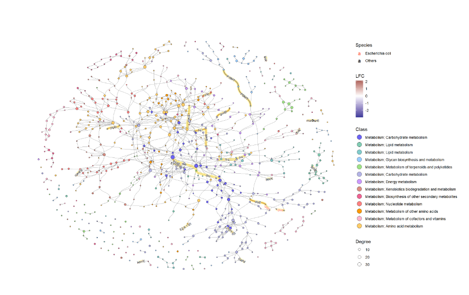
例子05-绘制通路富集全局图
使用 ko01100中的默认值和计算程度来可视化整个全局地图。
ggraph(g2, layout="fr")+
  geom_edge_link0(aes(color=I(fgcolor)), width=0.1)+
  geom_node_point(aes(fill=I(fgcolor), size=Degree), color="black", shape=21)+
  theme_graph()

为了有效地进行可视化,我们可以在 KEGG 路径中的各个组件上应用各种宝石图。在这个例子中,我们通过 ggfx 突出显示了由其 LFC 着色的重要边(KO) ,点大小对应于网络中的度,并且我们显示了重要 KO 名称的边标签。KO 名称由“物种”属性着色。这次我们把这个设置为大肠桿菌和其他。
ggraph(g2, layout="fr") +
  geom_edge_diagonal(color="grey50", width=0.1)+ ## Base edge
  ggfx::with_outer_glow(
    geom_edge_diagonal(aes(color=kolfc,filter=siglgl),
                       angle_calc = "along",
                       label_size=2.5),
    colour="gold", expand=3
  )+ ## Highlight significant edges
  scale_edge_color_gradient2(midpoint = 0, mid = "white",
                                    low=scales::muted("blue"),
                                    high=scales::muted("red"),
                                    name="LFC")+ ## Set gradient color
  geom_node_point(aes(fill=bgcolor,size=Degree),
                  shape=21,
                  color="black")+ ## Node size set to degree
  scale_size(range=c(1,4))+
  geom_edge_label_diagonal(aes(
    label=kon,
    label_colour=Species,
    filter=siglgl
  ),
  angle_calc = "along",
  label_size=2.5)+ ## Showing edge label, label color is Species attribute
  scale_label_colour_manual(values=c("tomato","black"),
                            name="Species")+ ## Scale color for edge label
  scale_fill_manual(values=hex,labels=class,name="Class")+ ## Show legend based on HEX
  theme_graph()+
  guides(fill = guide_legend(override.aes = list(size=5))) ## Change legend point size
## Subset and do the same thing
g2 |>
  morph(to_subgraph, siglgl) |>
  activate(nodes) |>
  mutate(tmp=centrality_degree(mode="all")) |>
  filter(tmp>0) |>
  mutate(subname=compn) |>
  unmorph() |>
  activate(nodes) |>
  filter(bgcolor=="#B3B3E6") |>
  mutate(Degree=centrality_degree(mode="all")) |> ## Calculate degree
  filter(Degree>0) |>
ggraph(layout="fr") +
  geom_edge_diagonal(color="grey50", width=0.1)+ ## Base edge
  ggfx::with_outer_glow(
    geom_edge_diagonal(aes(color=kolfc,filter=siglgl),
                       angle_calc = "along",
                       label_size=2.5),
    colour="gold", expand=3
  )+
  scale_edge_color_gradient2(midpoint = 0, mid = "white",
                             low=scales::muted("blue"),
                             high=scales::muted("red"),
                             name="LFC")+
  geom_node_point(aes(fill=bgcolor,size=Degree),
                  shape=21,
                  color="black")+
  scale_size(range=c(1,4))+
  geom_edge_label_diagonal(aes(
    label=kon,
    label_colour=Species,
    filter=siglgl
  ),
  angle_calc = "along",
  label_size=2.5)+ ## Showing edge label
  scale_label_colour_manual(values=c("tomato","black"),
                            name="Species")+ ## Scale color for edge label
  geom_node_text(aes(label=stringr::str_wrap(subname,10,whitespace_only = FALSE)),
    repel=TRUE, bg.colour="white", size=2)+
  scale_fill_manual(values=hex,labels=class,name="Class")+
  theme_graph()+
  guides(fill = guide_legend(override.aes = list(size=5)))

ggkegg更多及更详细的用法,请看:https://noriakis.github.io/software/ggkegg/index.html
为了方便的使用,我们基于机器翻译,将ggkegg帮助文档进行翻译。译文后续将提供给大家。
往期文章:
1. 复现SCI文章系列专栏
2. 《生信知识库订阅须知》,同步更新,易于搜索与管理。
3. 最全WGCNA教程(替换数据即可出全部结果与图形)
4. 精美图形绘制教程
5. 转录组分析教程
一个转录组上游分析流程 | Hisat2-Stringtie
小杜的生信筆記 ,主要发表或收录生物信息学的教程,以及基于R的分析和可视化(包括数据分析,图形绘制等);分享感兴趣的文献和学习资料!!


 5万+
5万+


 被折叠的 条评论
为什么被折叠?
被折叠的 条评论
为什么被折叠?
 到【灌水乐园】发言


