


 本文介绍了如何利用KITTI数据集中的64线激光雷达和相机进行深度信息投影,包括数据准备、代码解析和问题解决。作者还探讨了在无人船领域中,如何处理激光雷达数据稀疏的问题,以及如何结合图像信息进行多传感器融合。
最近学习了一些自动驾驶的相关的投影知识,结合自身,做了小小的改进,得到了想要的效果,故记录下来!
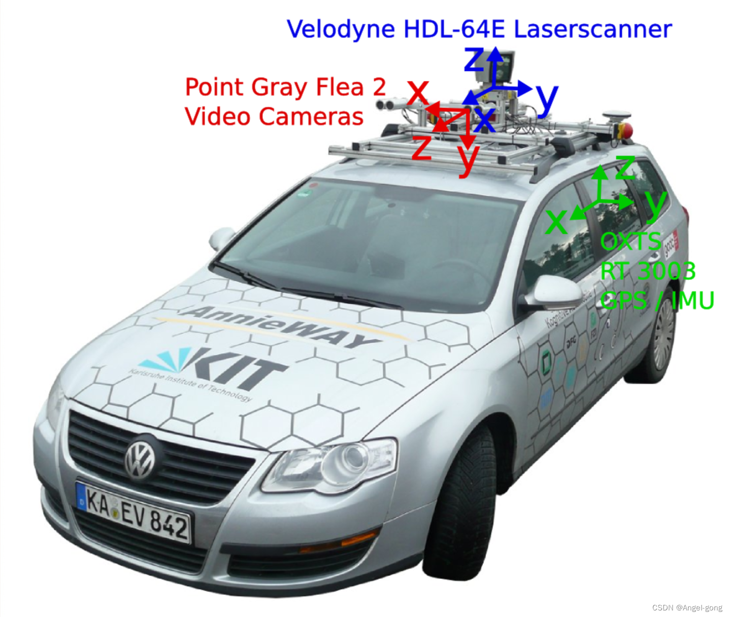
KITTI数据集介绍
1个64线激光雷达:车身正中间
2个GRB相机:得到RGB图像数据
2个灰度图像:得到灰度图像
激光雷达和相机的坐标系:
激光雷达:
x:前 y:左 z:上
相机:
x:右 y:下 z:前
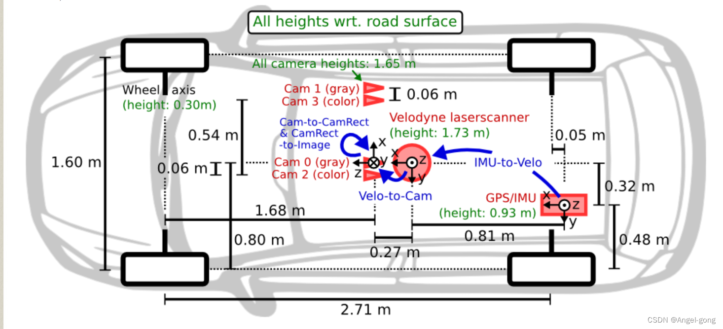
具体的安装位置(俯视图)如图:
更多详细介绍:

最近学习了一些自动驾驶的相关的投影知识,结合自身,做了小小的改进,得到了想要的效果,故记录下来!
1个64线激光雷达:车身正中间
2个GRB相机:得到RGB图像数据
2个灰度图像:得到灰度图像
激光雷达:
x:前 y:左 z:上
相机:
x:右 y:下 z:前
具体的安装位置(俯视图)如图:
更多详细介绍:
 2784
4110
2784
4110

 被折叠的 条评论
为什么被折叠?
被折叠的 条评论
为什么被折叠?
 到【灌水乐园】发言


 订阅专栏 解锁全文


