R语言绘制世界地图采样图

如果要发文章的话，可以做一个世界地图采样图（不知道是不是叫这个），显得数据量很足，有说服力，比如这样

https://www.cell.com/cell/fulltext/S0092-8674(19)30341-1?_returnURL=https%3A%2F%2Flinkinghub.elsevier.com%2Fretrieve%2Fpii%2FS0092867419303411%3Fshowall%3Dtrue#

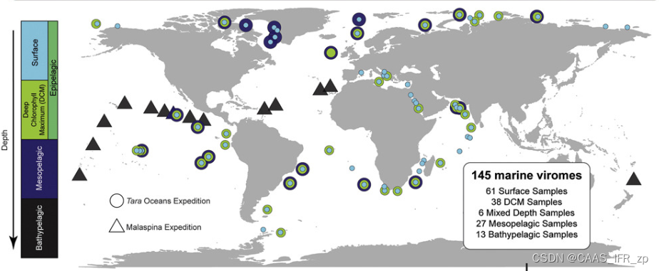
 看着很高级。今天我们来学习一下怎么用R语言绘制类似的图。

直接上代码

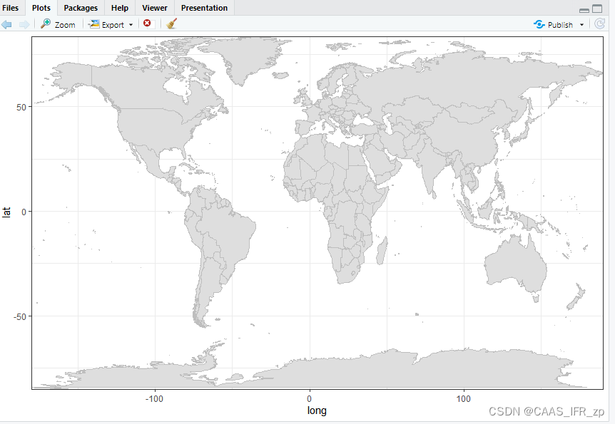
library(ggplot2)

world <- map_data("world")

ggplot() + 
    geom_polygon(data = world, aes(x = long, y = lat, group = group),
                 fill = "#dedede") +
    
    # 添加绘制国家边界线
    geom_path(data = world, aes(x = long, y = lat, group = group), 
              color = "grey", linewidth = 0.05) +
    
    theme_bw() +
    scale_y_continuous(expand = expansion(mult=c(0,0))) + 
    scale_x_continuous(expand = expansion(add=c(0,0)))

得到如下结果： 

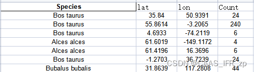
 准备经纬度信息和美化

如果纬度方向是北纬，就保持原来的数值，如果是南纬，就取相反数。

如果经度方向是东经，就保持原来的数值，如果是西经，就取相反数。

W - West 西经

E - East 东经

N - North 北纬

S - South 南纬

library(ggplot2)
library(sf)
library(ggalt)
library(viridis)
library(viridisLite)
library(RColorBrewer)

# 读取世界地图数据
world <- map_data("world")

# 读取自己的数据
data <- read.csv("C:/Users/fordata/Desktop/研究生/第一个想法(宏基因找病毒和肠型)/地理图.csv")

# 创建一个ggplot对象
g <- ggplot()

# 添加多边形图层，绘制世界地图
g <- g + geom_polygon(
    data = world, 
    aes(x = long, y = lat, group = group),
    fill = "#dedede"
)

# 添加路径图层，绘制国家边界线
g <- g + geom_path(
    data = world, 
    aes(x = long, y = lat, group = group), 
    color = "white", 
    linewidth = 0.05
)

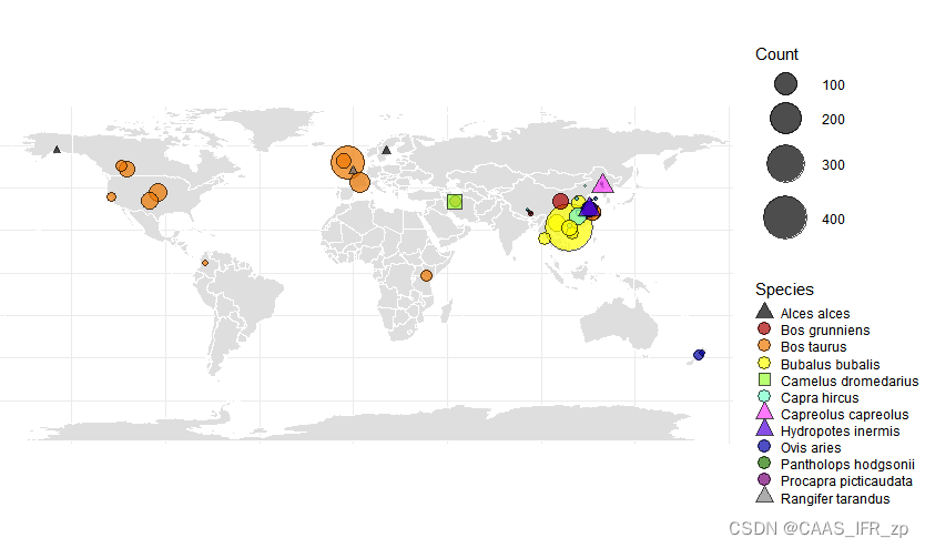
# 添加点图层，绘制自己的数据
g <- g + geom_point( data = data, aes(x = lon, y = lat, size = Count , fill = Species, shape = Species), alpha = 0.7, color = "black", stroke = 0.5 )

# 设置不同物种的颜色形状
g <- g + scale_fill_manual(
    values = c("#000000", "#AA0000", "#EE7700", "#FFFF00", "#99FF33", "#77FFCC", "#FF3EFF", "#5500DD", "#0000AA", "#227700", "#770077", "#888888")
)
g <- g + scale_shape_manual(values = c(24, 21, 21, 21, 22, 21, 24, 24, 21, 21, 21, 24))
# 设置黑白主题
g <- g + theme_bw()

# 设置坐标轴范围
g <- g + scale_y_continuous(expand = expansion(mult=c(0,0))) 
g <- g + scale_x_continuous(expand = expansion(add=c(0,0)))

# 隐藏坐标轴和网格线
g <- g + theme(
    axis.line    = element_blank(),
    axis.text.x  = element_blank(),
    axis.text.y  = element_blank(),
    axis.ticks   = element_blank(),
    axis.title.x = element_blank(),
    axis.title.y = element_blank(),panel.border = element_blank()
)

# 设置点的大小比例
g <- g + scale_size_area(max_size=15)

# 设置坐标系为 Robinson 投影
g <- g + coord_sf(crs= "+proj=robin +lon_0=0 +x_0=0 +y_0=0 +ellps=WGS84 +datum=WGS84 +units=m +no_defs")

# 设置图例中的圆的大小为4
g <- g + guides(fill=guide_legend(keywidth=0.1, keyheight=0.1,override.aes=list(size=4)))

g

#geom_point里加上show.legend = FALSE隐藏图例
ggsave("myplot.tiff", plot = g, device = "tiff", dpi = 300)

#geom_point里加删去show.legend = FALSE显示图例
library(gridExtra)
library(grid)
# 定义 g_legend() 函数
g_legend <- function(a.gplot){
  tmp <- ggplot_gtable(ggplot_build(a.gplot))
  leg <- which(sapply(tmp$grobs, function(x) x$name) == "guide-box")
  legend <- tmp$grobs[[leg]]
  return(legend)
}
# 提取图例
legend <- g_legend(g)
# 绘制图例
grid.newpage()
grid.draw(legend)
ggsave("legend.tiff", plot = legend, device = "tiff", dpi = 300)