机器学习：支持向量机

最新推荐文章于 2024-07-10 17:21:21 发布

山问信未临

最新推荐文章于 2024-07-10 17:21:21 发布

阅读量819

点赞数 8

分类专栏：机器学习文章标签：机器学习支持向量机人工智能

本文链接：https://blog.csdn.net/m0_71146337/article/details/136127525

版权

机器学习专栏收录该内容

9 篇文章 2 订阅

订阅专栏

介绍

在本实验中，将使用支持向量机(Support Vector Machine, SVM)并了解其在数据上的工作原理。

本次实验需要用到的数据集包括：

Exp_data1.mat -线性SVM分类数据集
Exp_data2.mat -高斯核SVM分类数据集
Exp_data3.mat -搜索最优参数高斯核SVM分类数据集

评分标准如下：

要点1：使用线性SVM-----------------（20分）
要点2：定义高斯核---------------------（20分）
要点3：使用高斯核SVM---------------（20分）
要点4：搜索SVM最优参数------------（20分）
要点5：手写体数字识别---------------（20分）

# 引入所需要的库文件
import numpy as np
import pandas as pd
import matplotlib.pyplot as plt
from scipy.io import loadmat
import os


%matplotlib inline

1 线性SVM

在该部分实验中，将实现线性SVM分类并将其应用于数据集1。

raw_data = loadmat('Exp_data1.mat')
data = pd.DataFrame(raw_data.get('X'), columns=['X1', 'X2'])
data['y'] = raw_data.get('y')
data.drop(data.tail(1).index,inplace=True)
data.head()

X=data[['X1', 'X2']]
y=data['y']
X=X.to_numpy()
y=y.to_numpy()

# 定义数据可视化函数 
def plot_init_data(data, fig, ax):
    positive = data[data['y'].isin([1])]
    negative = data[data['y'].isin([0])]

    ax.scatter(positive['X1'], positive['X2'], s=50, marker='x', label='Positive')
    ax.scatter(negative['X1'], negative['X2'], s=50, marker='o', label='Negative')

# 数据可视化
fig, ax = plt.subplots(figsize=(9,6))
plot_init_data(data, fig, ax)
ax.legend()
plt.show()

**要点 1：** 通过调用sklearn中的svm.LinearSVC函数实现SVM，要求输出： 1. 分类精度 2. 前5个样本的预测值 (f(x)=wTx+b)(�(�)=��+�) 3. 支持向量指标(满足1≤f(x)≤1+e−41≤�(�)≤1+�−4的样本可认为是支持向量) 4. 支持向量建议参数：C=1e3, loss='hinge', max_iter=1e5, random_state=0 参考结果为：分类精度： 1.0 前5个样本预测值： [2.78 1.31 5.26 2.04 1.54] 支持向量指标： [11 12 47] 支持向量： [[3.1 3.07] [1.92 4.05] [2.54 2.89]]

# ====================== 在这里填入代码 ======================= 
from sklearn import svm
clf = svm.LinearSVC(C=1e3, loss='hinge', max_iter=1e5, random_state=0)
clf.fit(X, y)
acc = clf.score(X, y)
pred = clf.decision_function(X)
support_vector_indices =np.where(np.abs(pred)<=1+np.e**(-4))[0]
support_vectors = X[support_vector_indices]
# ============================================================= 
print('分类精度：\n', np.around(acc,decimals=2))
print('前5个样本预测值：\n', np.around(pred[0:5],decimals=2))
print('支持向量指标：\n', support_vector_indices)
print('支持向量：\n', np.around(support_vectors,decimals=2))

#可视化分类决策面和支持向量

from sklearn.inspection import DecisionBoundaryDisplay

fig, ax = plt.subplots(figsize=(9,6))
plot_init_data(data, fig, ax)
ax.legend()
ax = plt.gca()
DecisionBoundaryDisplay.from_estimator(
    svc,
    X,
    ax=ax,
    grid_resolution=50,
    plot_method="contour",
    colors="k",
    levels=[-1, 0, 1],
    alpha=1,
    linestyles=["--", "-", "--"],
    )
plt.scatter(
    support_vectors[:, 0],
    support_vectors[:, 1],
    s=200,
    linewidth=2,
    facecolors="none",
    edgecolors="r",
    )
plt.xlim(0.6, 4.1)
plt.show()

2 高斯核 SVM

在本部分实验中，将利用核SVM实现非线性分类任务。

2.1 高斯核

对于两个样本 $x_1$ , $x_2$ ∈ $R^d$ ，其高斯核定义为

$K_{gaussian}(x_1,x_2)=exp(-\frac{\left \| x_1-x_2 \right \|_2^2}{2\sigma ^2})$

**要点 2：** 本部分的任务为按照上述公式实现高斯核函数的定义。

def gaussianKernel(x1, x2, sigma):
    """
    定义高斯核.
    
    输入参数
    ----------
    x1 :  第一个样本点，大小为(d,1)的向量
    
    x2 :  第二个样本点，大小为(d,1)的向量
    
    sigma : 高斯核的带宽参数

    输出结果
    -------
    sim : 两个样本的相似度 (similarity)。
    
    """
# ====================== 在这里填入代码 ======================= 

    dist = np.linalg.norm(x1 - x2)
    sim = np.exp(-dist**2 / (2 * sigma**2))

# ============================================================= 
    return sim

如果完成了上述的高斯核函数 gaussianKernel，以下代码可用于测试。如果结果为0.32，则计算通过。

#测试高斯核函数
x1 = np.array([1, 2, 1])
x2 = np.array([0, 4, -1])
sigma = 2
sim = gaussianKernel(x1, x2, sigma)
 
print('Gaussian Kernel between x1  and x2 is :', np.around(sim,decimals=2))

2.2 高斯核SVM应用于数据集2

在本部分实验中，将高斯核SVM应用于数据集2：Exp_data2.mat。

raw_data = loadmat('Exp_data2.mat')

data = pd.DataFrame(raw_data['X'], columns=['X1', 'X2'])
data['y'] = raw_data['y']

fig, ax = plt.subplots(figsize=(9,6))
plot_init_data(data, fig, ax)
ax.legend()
plt.show()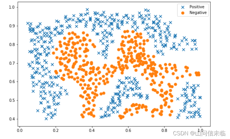

从上图中可看出，上述两类样本是线性不可分的。需要采用核SVM进行分类。

**要点 3：** 本部分的任务为使用高斯核SVM于数据集2。可调用sklearn库实现非线性SVM函数svm.SVC。

# ====================== 在这里填入代码 ======================= 
X = data[['X1', 'X2']]
y = data['y']
clf = svm.SVC(kernel='rbf', gamma=1)
clf.fit(X, y)
score = clf.score(X, y)
    
# ============================================================= 
print("最优参数对应的分类精度:", np.around(score,decimals=3)) 


#可视化
X=data[['X1', 'X2']].to_numpy()
x1,x2 = np.meshgrid(np.linspace(X[:,0].min(),X[:,1].max(),num=150),np.linspace(X[:,1].min(),X[:,1].max(),num=150))
fig, ax = plt.subplots(figsize=(9,6))
plot_init_data(data, fig, ax)
plt.contour(x1,x2,clf.predict(np.array([x1.ravel(),x2.ravel()]).T).reshape(x1.shape),2,colors="g")
ax.legend()
plt.show()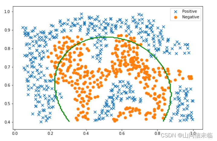

3 搜索SVM最优参数

在本部分实验中，将通过交叉验证方法选择高斯核SVM的最优参数C�和σ�，并将其应用于数据集3：Exp_data3.mat。该数据集包含训练样本集X（训练样本特征）, y（训练样本标记）和验证集 Xval（验证样本特征）, yval（验证样本标记）。

raw_data = loadmat('Exp_data3.mat')

X = raw_data['X']
Xval = raw_data['Xval']
y = raw_data['y'].ravel()
yval = raw_data['yval'].ravel()

fig, ax = plt.subplots(figsize=(9,6))
data = pd.DataFrame(raw_data.get('X'), columns=['X1', 'X2'])
data['y'] = raw_data.get('y')
plot_init_data(data, fig, ax)
plt.show()

3.1 搜索SVM最优参数 C� 和 σ�

**要点 4：**本部分的任务为搜索高斯SVM最优参数C�和σ�。对于C�和σ�，可从以下候选集合中搜索 {0.01,0.03,0.1,0.3,1,3,10,30}

C_values = [0.01, 0.03, 0.1, 0.3, 1, 3, 10, 30, 100]
gamma_values = [0.01, 0.03, 0.1, 0.3, 1, 3, 10, 30, 100]
best_score = 0
# ====================== 在这里填入代码 ======================= 
for C in C_values:
    for gamma in gamma_values:
        clf = svm.SVC(C=C, kernel='rbf', gamma=gamma)
        clf.fit(X, y)
        score = clf.score(Xval, yval)
        if score > best_score:
            best_score = score
            best_C = C
            best_gamma = gamma

# ============================================================= 
print("最优参数C:", np.around(best_C,decimals=3)) 
print("最优参数gamma:", np.around(best_gamma,decimals=3)) 
print("最优参数对应的分类精度:", np.around(best_score,decimals=3))

3.2 利用已选出的参数和高斯核SVM应用于数据集3

svc = svm.SVC(C=best_C, gamma=best_gamma,max_iter=1e3)
svc.fit(X, y)
x1,x2 = np.meshgrid(np.linspace(X[:,0].min(),X[:,1].max(),num=150),np.linspace(X[:,1].min(),X[:,1].max(),num=150))
fig, ax = plt.subplots(figsize=(9,6))
plot_init_data(data, fig, ax)
plt.contour(x1,x2,svc.predict(np.array([x1.ravel(),x2.ravel()]).T).reshape(x1.shape),2,colors="g")
ax.legend()
plt.xlim(-0.65,0.35)
plt.show()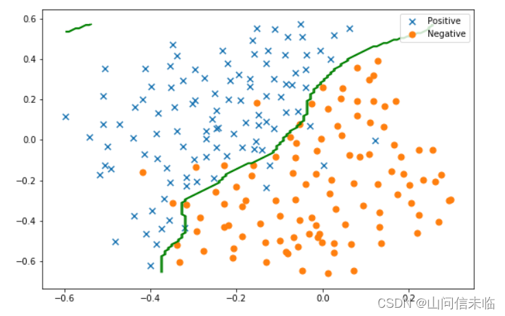

4 将 SVM 应用于手写体数字识别

在本部分实验中，将线性SVM和高斯核SVM应用于手写体数据集：UCI ML hand-written digits datasets，并对比识别结果。

# 引入所需要的库文件
from sklearn import datasets, svm, metrics
from sklearn.model_selection import train_test_split
# 从sklearn库中下载数据集并展示部分样本
digits = datasets.load_digits()

_, axes = plt.subplots(1, 10) 
images_and_labels = list(zip(digits.images, digits.target))
for ax, (image, label) in zip(axes, images_and_labels[0:10]):
    ax.set_axis_off()
    ax.imshow(image, cmap=plt.cm.gray_r, interpolation='nearest')
    ax.set_title(' %i' % label)
plt.show()
#将每个图片样本变成向量
n_samples = len(digits.images)
data = digits.images.reshape((n_samples, -1))

# 将原始数据集划分成训练集和测试集（一半训练，另一半做测试）
X_train, X_test, y_train, y_test = train_test_split(
    data, digits.target, test_size=0.5, shuffle=False)#False

**要点 5：** 本部分的任务为将线性SVM（C=1）和高斯核SVM（C=1, gamma=0.001）应用于UCI手写体数据集并输出识别精度。

#将线性SVM应用于该数据集并输出识别结果
# ====================== 在这里填入代码 ======================= 
 
clf = svm.LinearSVC(C=1)
clf.fit(X_train, y_train)
score_Linear = clf.score(X_test, y_test)
    
    
# ============================================================= 
 
print("线性SVM分类精度:", np.around(score_Linear,decimals=2)) 


#将高斯核SVM应用于该数据集并输出识别结果
# ====================== 在这里填入代码 ======================= 
 
    
clf = svm.SVC(C=1, kernel='rbf', gamma=0.001)
clf.fit(X_train, y_train)
score_Gaussian = clf.score(X_test, y_test)  
    
# ============================================================= 
print("高斯SVM分类精度:", np.around(score_Gaussian,decimals=2))

山问信未临

关注

8
点赞
踩
8

收藏

觉得还不错? 一键收藏
1
评论
机器学习：支持向量机

在本实验中，将使用支持向量机(Support Vector Machine, SVM)并了解其在数据上的工作原理。本次实验需要用到的数据集包括：Exp_data1.mat -线性SVM分类数据集Exp_data2.mat -高斯核SVM分类数据集Exp_data3.mat -搜索最优参数高斯核SVM分类数据集
复制链接

扫一扫