scRNA-seq | 吐血整理的单细胞入门教程（数据格式和处理）（四）

写在前面

我们还是在正式进行代码操作前想几个小问题：👇

• 如何将单细胞数据导入R中？
• 不同类型的数据/信息（如细胞信息、基因信息等）是如何存储和操作的？
• 如何获得细胞和基因的基本信息并对数据进行相应的过滤？

用到的包

目前常用的scRNA-seq分析包，包括Seurat、Scanpy(python)、Scater、Monocle2、Monocle3等。🤒

rm(list = ls())
library(tidyverse)
library(SingleCellExperiment)
library(DropletUtils)

数据格式

scRNA-seq的标准格式为SingleCellExperiment。 😘
Note! Seurat包有其自己的格式，即Seurat格式，可能因为Seurat太火了吧，越来越多的包都开始兼容Seurat格式的文件了。😂

我们拿到的数据通常是一个feature-by-sample的表达矩阵。
在scRNA-seq分析中，我们一般需要从counts矩阵开始分析，代表每个cell的feature的reads/UMI。feature可以是gene、isoforms或exons。🤒

SingleCellExperiment对象

4.1 读入数据

counts <- read.table("./molecules.txt", sep = "\t")
annotation <- read.table("./annotation.txt", sep = "\t", header = TRUE)

---

4.2 创建SingleCellExperiment对象

# 注意assays必须是matrix
tung <- SingleCellExperiment(
  assays = list(counts = as.matrix(counts)),
  colData = annotation
)

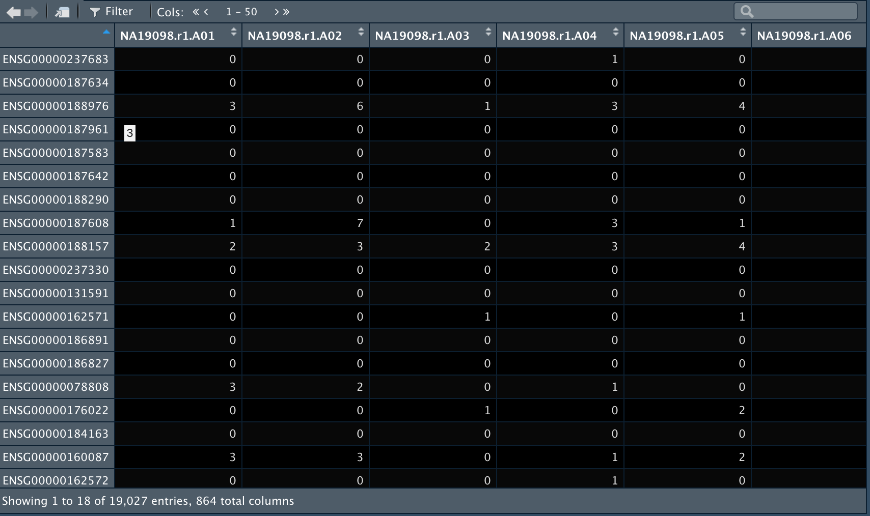
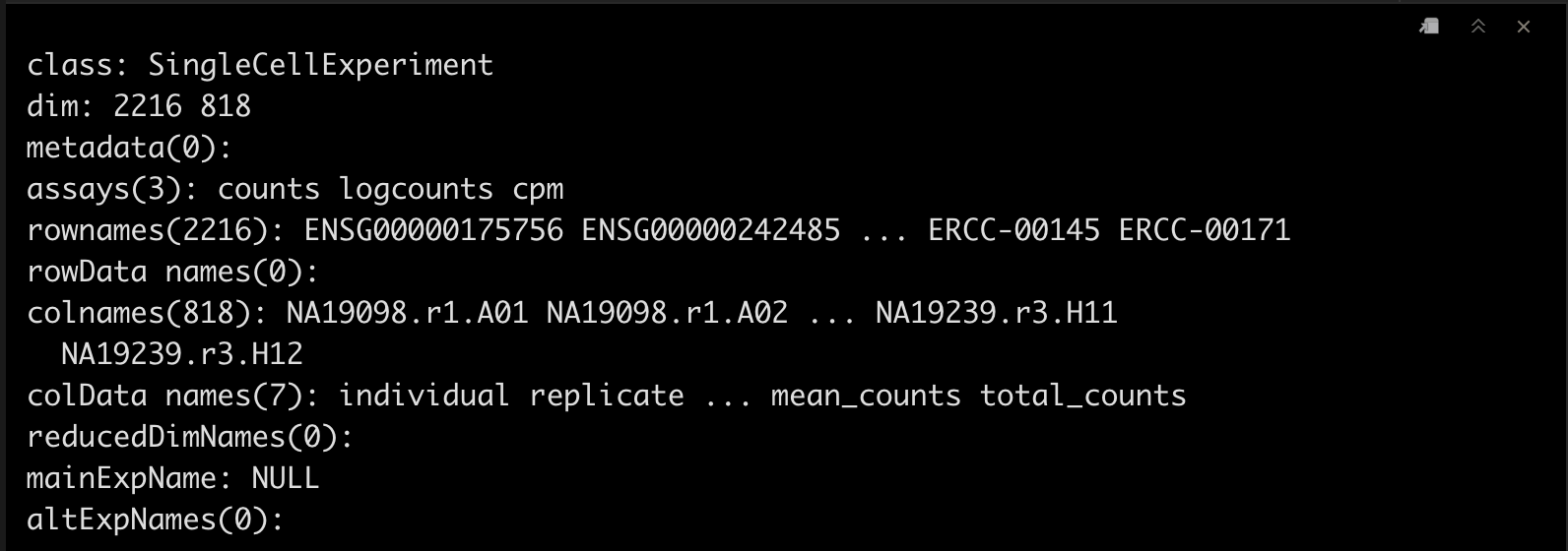
tung

Note! 这个SingleCellExperiment包含：

• 19027个基因(行)和864个细胞(列);
• 一个名为counts的assays;
• 预览部分基因名(rownames)和细胞名(colnames);
• 基因的metadata为空 (rowData);
• 细胞的metabdata(colData names)

10X 文件的读取

像上面那样创建SingleCellExperiment对象,几乎适用于任何情况，我们只需要一个counts矩阵即可。 🤗
但有时候我们获取的文件是cellranger（用于10X Chromium数据）的输出文件，这个时候我们可以用DropletUtils包中的read10xCounts函数。😀

sce <- read10xCounts("./pbmc_1k_raw")

sce <- read10xCounts("./pbmc_1k_filtered")
sce

查看数据

6.1 查看counts矩阵

这里需要说一下的是，如果你的矩阵就叫counts,那么counts(tung) = assay(tung, "counts")。

counts(tung)
assay(tung, "counts")[1:4,1:4]

---

6.2 查看cell信息

colData(tung)

---

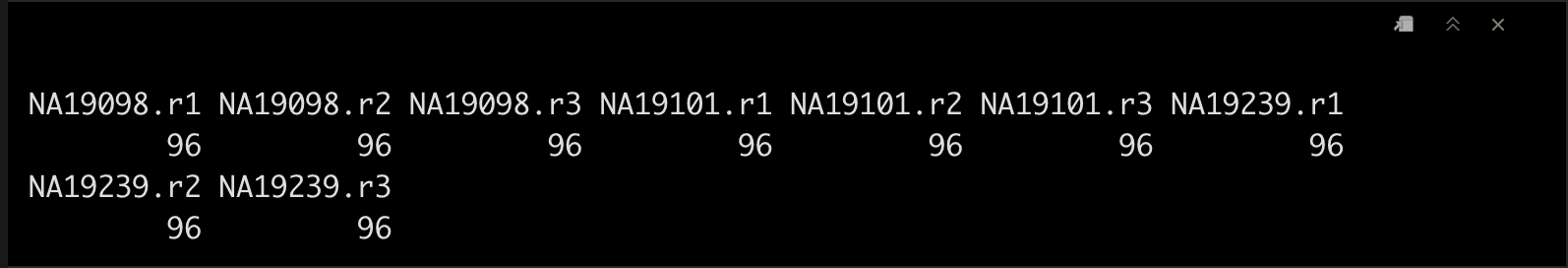
6.3 查看batch信息

table(tung$batch)

---

🧐 补充！

Function	Description
rowData(sce)	gene信息
colData(sce)	cell信息
assay(sce, "counts")	查看counts矩阵
reducedDim(sce, "PCA")	查看PCA降维table
sce$colname	查看colData的colname, 等价于colData(sce)$colname
sce[<rows>, <columns>]	查看特定行、列

修改SingleCellExperiment对象

举个栗子 🌰
我们把counts矩阵进行log2(x+1)转换，命名为logcounts。

assay(tung, "logcounts") <- log2(counts(tung) + 1)
# 查看一下
logcounts(tung)[1:4, 1:4] 

---

🧐 补充！

Code	Description
assay(sce, "name") <- matrix	添加新矩阵
rowData(sce) <- data_frame	替换rowData
colData(sce) <- data_frame	替换colData
colData(sce)$column_name <- values	在colData中添加/替换一个新的列
rowData(sce)$column_name <- values	在rowData中添加/替换一个新的行
reducedDim(sce, "name") <- matrix	添加降维矩阵

基本数据处理

8.1 举个栗子🌰

计算我们的数据集中每个细胞（列）的平均counts。
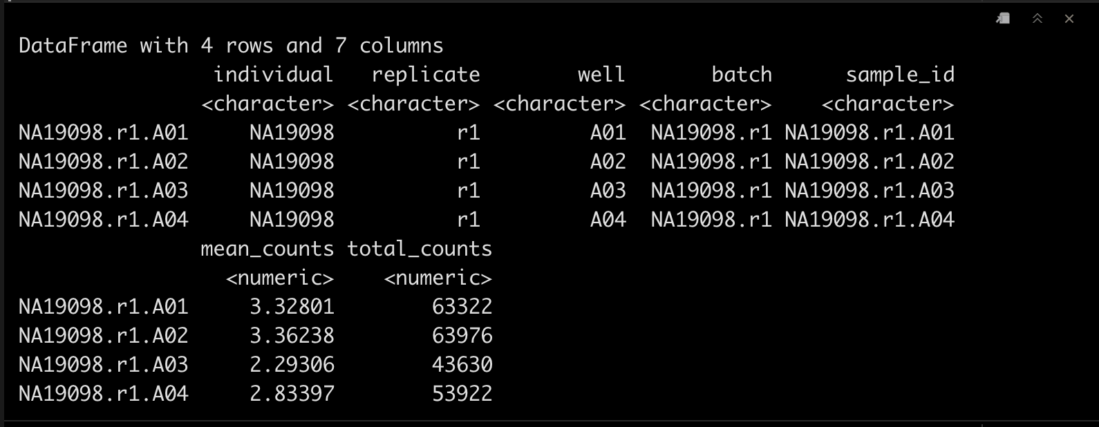
然后我们将它加到column metadata中作为新的一列。😘

colData(tung)$mean_counts <- colMeans(counts(tung))

---

这个时候我们可以查看一下，多了一列mean_counts。🤔

colData(tung)[1:4,]

---

8.2 补充一下

这里我们再补充一下基本函数。有兴趣的小伙伴都试试吧。🫶

• row (feature) summaries

rowSums(counts(tung))  # sum
rowMeans(counts(tung)) # mean
rowSds(counts(tung))   # standard deviation
rowVars(counts(tung))  # variance
rowIQRs(counts(tung))  # inter-quartile range
rowMads(counts(tung))  # mean absolute deviation

---

• column (sample) summaries

colSums(counts(tung))  # sum
colMeans(counts(tung)) # mean
colSds(counts(tung))   # standard deviation
colVars(counts(tung))  # variance
colIQRs(counts(tung))  # inter-quartile range
colMads(counts(tung))  # mean absolute deviation

---

CPM的计算与查看

9.1 CPM的计算

这里我们直接使用sweep函数来搞定counts转CPM，在这之前我们先计算一下total counts并新增一列。

colData(tung)$total_counts <- colSums(counts(tung))
assay(tung, "cpm") <- sweep(counts(tung),2,tung$total_counts/1e6,'/')

# check一下
colSums(cpm(tung))[1:10]

---

9.2 CPM矩阵的查看

cpm(tung)[1:4, 1:4]
assay(tung, "cpm")[1:4, 1:4]

常用过滤方法

拿到矩阵后，我们一般需要过滤一些低表达或异常表达值。
举个栗子 🌰，假设细胞至少25000counts，基因在至少一半的细胞中拥有超过5个counts。

10.1 过滤细胞

cell_filter <- colSums(counts(tung)) >= 25000

# check一下
table(cell_filter)

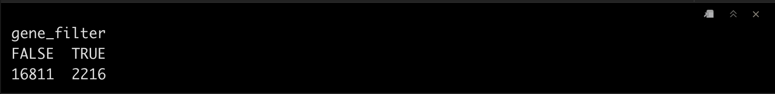
10.2 过滤基因

gene_filter <- rowSums(counts(tung) > 5) > ncol(tung)/2

# check一下
table(gene_filter)

10.3 最终过滤

tung_filtered <- tung[gene_filter, cell_filter]

tung_filtered

---

10.4 补充一下

colSums(counts(sce)) > x # 对细胞进行过滤, Total counts per cell greater than x。

colSums(counts(sce) > x) > y # 对细胞进行过滤，Cells with at least y genes having counts greater than x.

rowSums(counts(sce)) > x # 对基因进行滤过，Total counts per gene greater than x.

rowSums(counts(sce) > x) > y # 对基因进行过滤，Genes with at least y cells having counts greater than x.

---

最后祝大家早日不卷!~

---

需要示例数据的小伙伴，在公众号回复scRNAseq获取吧！

点个在看吧各位~ ✐.ɴɪᴄᴇ ᴅᴀʏ 〰

本文由mdnice多平台发布