


1 内容介绍
莱斯分布实际上可以理解为主信号与服从瑞利分布的多径信号分量的和。概率密度函数公式中,R即为正弦(余弦)信号加窄带高斯随机信号的包络,参数A是主信号幅度的峰值,σ^2是多径信号分量的功率,I0()是修正的0阶第一类贝塞尔函数。
是不是感觉这个更抽象了,那有什么用呢,在通信中,有一个信号占主要成分的噪声中,信道噪声一般呈现莱斯分布。
2 部分代码
clear;clc;
close all
%% Parameters
N = 1e5;
b = 0.279;
m = 2;
Omega = 0.251;
%% Generate Shadowed Rician Random Number
X = ShadowedRicianRandGen(b,m,Omega,N);
%% Points for which distribution has to be evaluated
x = linspace(0,5,1000);
%% Estimate Distribution
[fsim,Fsim] = EstimateDistribution(X,x);
%% Theoretical PDF & CDF
[fana,Fana] = ShadowedRicianDistribution(b,m,Omega,x);
%% Plot Results
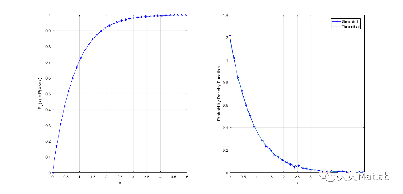
subplot(121);plot(x(1:30:end),Fsim(1:30:end),'-b*',x,Fana,'-');grid on;
xlabel('x');ylabel('F_X(x) = P(X<=x)');
subplot(122);plot(x(1:30:end),fsim(1:30:end),'-b*',x,fana,'-');grid on;
xlabel('x');
ylabel('Probability Density Function');
legend('Simulated','Theoretical');
function X = ShadowedRicianRandGen(b,m,Omega,N,a)
% This function generates random number according to shadowed Rician
% density function.
%
% INPUTS:
% b = Scalar (real), Average power of multipath component
% m = Scalar (real), Fading severity parameter
% Omega = Scalar (real), Average power of LOS component
% N = Scalar (real) specifying number of random number to be
% generated
% OUTPUTS:
% X = Scalar (Column Vector if N > 1) specifying random number
% generated using Shadowed Rician distribution function
%
% USAGE EXAMPLES:
% X = ShadowedRicianRandGen(0.279,2,0.251);
%
% REFERENCES:
% A. Abdi, W. C. Lau, M.-S. Alouini, and M. Kaveh, 揂 new simple model
% for land mobile satellite channels: First- and second-order statistics,?% IEEE Trans. Wireless Commun., vol. 2, no. 3, pp. 519?28, May 2003.
% Jeruchim, M. C., P. Balaban, and K. S. Shanmugam, Simulation of
% Communication Systems, New York, Plenum Press, 1992.
%
% Implemented By:
% Ashish (MEET) Meshram
% meetashish85@gmail.com;
% Checking Input Arguments
if nargin<5||isempty(a),a = 10;end
if nargin<4||isempty(N),N = 10000;end
if nargin<3||isempty(Omega)
error('Missing Input Argument: Please specify omega');
end
if nargin<2||isempty(m)
error('Missing Input Argument: Please specify m');
end
if nargin<1||isempty(b)
error('Missing Input Argument: Please specify b');
end
% Implementation Starts Here
X = zeros(N,1); % Preallocating memory space for X
% Intermediate Variables
alpha = ((2*b*m)/(2*b*m + Omega))^m;
beta = Omega/(2*b*(2*b*m + Omega));
lambda = 1/(2*b);
% Maximum value of Shadowed Rician value occurs at x = 0;
maxfx = alpha*lambda;
c = maxfx;
% Accept and Reject Algorithm
for k = 1:N
accept = false;
while accept == false
U2 = c*rand; % Generating U2, Uniformly disributed
% random number [0,c]
U1 = a*rand; % Generating U1, Uniformly distributed
% in [0,a]
% Evaluating fx for U1
fx = alpha*lambda*exp(-U1*lambda)*Kummer(m,1,beta*U1);
% if U2 is less than or equal to fx at U1 then its taken as X else
% repeat the above procedure
if U2 <= fx
X(k) = U1;
accept = true;
end
end
end
function y = Kummer(a,b,z,maxit)
% This function implements 1F1(.;.;.), Confluent Hypergeometric function.
%
% INPUTS:
% a = Scalar and complex
% b = Scalar and complex
% z = Scalar and complex
% maxit = Scalar and real number specifying maximum number of iteration.
% Default, maxit = 5;
%
% OUTPUT:
% y = Scalar and complex
%
% Implemented By:
% Ashish (MEET) Meshram
% meetashish85@gmail.com;
% Checking Input Arguments
if nargin<1||isempty(a)
error('Missing Input Argument: Please specify a');
end
if nargin<2||isempty(b)
error('Missing Input Argument: Please specify b');
end
if nargin<3||isempty(z)
error('Missing Input Argument: Please specify z');
end
if nargin<4||isempty(maxit),maxit = 5;end
% Implementation
ytemp = 1;
for k = 1:maxit
ytemp = ytemp...
+ PochhammerSymbol(a,k)/(PochhammerSymbol(b,k)...
* factorial(k))*z^k;
y = ytemp;
end
function y = PochhammerSymbol(x,n)
if n == 0
y = 1;
else
y = 1;
for k = 1:n
y = y*(x + k - 1);
end
end
function [f,F] = EstimateDistribution(X,x)
% This function implements estimation of CDF and PDF of one dimensional
% random variables.
%
% INPUTS:
% X = vector specifying random variables
% x = vector specifying points for which CDF and PDF has to be
% evaluated
% OUTPUTS:
% f = vector specifying estimated PDF of random variable X for
% points.
% F = vector specifying estimated CDF of random variable X for
% points.
%
% USAGE EXAMPLES:
% %% Generate N Standard Normally Distributed Random Variable
% N = 1000000;
% X = randn(N,1);
% %% Points for which CDF and PDF are to be evaluated
% x = linspace(-10,10,1000);
% %% Estimate PDF and CDF
% [f,F] = EstimateDistribution(X,x);
% %% Plot Results
% figure(1);
% plot(x,f,x,F);
% xlabel('x');
% ylabel('Simulated PDF & CDF');
% str1 = strcat('PDF;','Area = ',num2str(trapz(x,f)));
% legend(str1,'CDF','Location','northwest');
%
%
% %% Generate N Gaussianly Distributed Random Variable with specific mean and
% %% Standard Deviation
% N = 1000000;
% mu = -1;
% sigma = 5;
% X = mu + sigma*randn(N,1);
% %% Points for which CDF and PDF are to be evaluated
% x = linspace(-10,10,1000);
% %% Theoretical PDF and CDF
% fx = (1/sqrt((2*pi*sigma*sigma)))*exp(-(((x - mu).^2)/(2*sigma*sigma)));
% Fx = 0.5*(1 + erf((x - mu)/(sqrt(2*sigma*sigma))));
% %% Estimate PDF and CDF
% [f,F] = EstimateDistribution(X,x);
% %% Plot Results
% figure(2);
% plot(x,f,x,fx,x,F,x,Fx);
% xlabel('x');
% ylabel('PDF & CDF');
% str1 = strcat('Simulated PDF;','Area = ',num2str(trapz(x,f)));
% str2 = strcat('Theoretical PDF;','Area = ',num2str(trapz(x,fx)));
% legend(str1,str2,'Simulated CDF','Theoretical CDF','Location','northwest');
%
%
% %% Generate N Uniformaly Distributed Random Variable
% N = 1000000;
% X = rand(N,1);
% %% Points for which CDF and PDF are to be evaluated
% x = linspace(-10,10,1000);
% %% Estimate PDF and CDF
% [f,F] = EstimateDistribution(X,x);
% %% Plot Results
% figure(3);
% plot(x,f,x,F);
% xlabel('x');
% ylabel('Simulated PDF & CDF');
% str1 = strcat('PDF;','Area = ',num2str(trapz(x,f)));
% legend(str1,'CDF','Location','northwest');
%
% REFERENCES:
% Athanasios Papoulis, S. Unnikrishna Pillai, Probability, Random Variables
% and Stochastic Processes, 4e
% Peyton Z. Peebles Jr., Probability, Random Variables, And Random Signal
% Principles, 2e
% Saeed Ghahramani, Fundamentals of Probability, with Stochastic Processes,
% 3e
%
% SEE ALSO:
% interp1, smooth
%
% AUTHOR:
% Ashish (Meet) Meshram
% meetashish85@gmail.com; mt1402102002@iiti.ac.in
% Checking Input Arguments
if nargin<2||isempty(x), x = linspace(-10,10,1000);end
if nargin<2||isempty(X)
error('Missing Input Arguments: Please specify vector random variables');
end
% Impelementation Starts Here
f = zeros(1,length(x)); % Preallocation of memory space
F = f; % Preallocation of memory space
h = 0.000000001; % Small value closer to zero for evaluating
% numerical differentiation.
% Estimating CDF by its definition
for m = 1:length(x)
p = 0; % True Probability
q = 0; % False Probability
for n = 1:length(X)
if X(n)<=x(m) % Definition of CDF
p = p + 1;
else
q = q + 1;
end
end
F(m) = p/(p + q); % Calulating Probability
end
% Estimating PDF by differentiation of CDF
for k = 1:length(x)
fxph = interp1(x,F,x(k) + h,'spline'); % Interpolating value of F(x+h)
fxmh = interp1(x,F,x(k) - h,'spline'); % Interpolating value of F(x-h)
f(k) = (fxph - fxmh)/(2*h); % Two-point formula to compute
end % Numerical differentiation
f = smooth(f); % Smoothing at last
function [f,F] = ShadowedRicianDistribution(b,m,Omega,x)
lambda = 1/(2*b);
alpha = (2*b*m)/(2*b*m + Omega);
beta = Omega/(2*b*(2*b*m + Omega));
% Theoretical PDF
f = zeros(length(x),1);
for k = 1:length(x)
f(k) = (alpha^m)*lambda*exp(-x(k)*lambda)*Kummer(m,1,beta*x(k));
end
% Theoretical CDF
sumk = zeros(500,1);
F = zeros(length(x),1);
for p = 1:length(x)
for q = 1:500
mmk = gamma(m+k);
mk = gamma(m);
betabylambdak = (beta/lambda)^k;
gammak = gammainc(k+1,lambda*x(p));
sumk(q) = (mmk/(mk*(factorial(k))^2))*betabylambdak*gammak;
end
F(p) = alpha*sum(sumk);
end
3 运行结果
4 参考文献
博主简介:擅长智能优化算法、神经网络预测、信号处理、元胞自动机、图像处理、路径规划、无人机、雷达通信、无线传感器等多种领域的Matlab仿真,相关matlab代码问题可私信交流。
部分理论引用网络文献,若有侵权联系博主删除。


 277
277

 被折叠的 条评论
为什么被折叠?
被折叠的 条评论
为什么被折叠?
 到【灌水乐园】发言


