YOLO+Sort实现目标追踪

在前面的目标检测、实例分割的学习中，我们多是对单张图像进行处理，而事实上在我们的实际应用中多数需要对视频进行操作，当然这个操作也是讲视频转换为一帧帧的图像，但博主发现在ultralytics这个算法平台中，针对视频的处理多调用track方法，即跟踪算法，比如在车辆测速、车辆测距等应用中，那么跟踪算法到底是如何实现的呢，这便是我们今天要学习的内容。

目标检测和目标跟踪的区别

• 目标检测:目标检测任务要求同时完成对象的定位（即确定对象的边界框位置）和分类（即确定对象的类别）。这意味着目标检测算法必须不仅能够确定对象是否存在，还要知道它是什么。
  目标检测通常用于识别和定位图像或视频帧中的对象，通常需要明确的目标类别信息。
• 目标跟踪:目标跟踪任务更关注对象在帧与帧之间的连续性，通常更注重对象的运动特征，而不要求进行目标的分类。
  目标跟踪可以不涉及目标的类别，它的主要目标是维护对象的位置和轨迹，以实现在视频序列中的跟踪。

现有的目标追踪方法，都是基于目标检测进行的，其中最主要的便是Sort目标追踪方法，这里就有个问题，视频中不同时刻的同一个人，位置发生了变化，那么是如何关联上的呢？答案就是匈牙利算法和卡尔曼滤波。

• 匈牙利算法可以告诉我们当前帧的某个目标，是否与前一帧的某个目标相同。
• 卡尔曼滤波可以基于目标前一时刻的位置，来预测当前时刻的位置，并且可以比传感器（在目标跟踪中即目标检测器，比如Yolo等）更准确的估计目标的位置。

IOU追踪器

所谓的追踪器，就是要保证帧与帧图像中目标的关联性，其中，最简单的追踪器便是IOU追踪器。
定义追踪器，并设置要追踪的类别以及IOU阈值

这种方法并没有涉及追踪器的预测，只是将检测结果存储在追踪器中，由此来判断两者是否匹配，即保证上一帧的检测结果与下一帧的检测结果匹配 成功即可。

代码如下：

'''
iou追踪示例
'''
from ultralytics import YOLO
import cv2
import time

class IouTracker:
    def __init__(self):

        # 加载检测模型
        self.detection_model = YOLO("../detection/yolov8n.pt")
        # 获取类别
        self.objs_labels = self.detection_model.names
        # 打印类别
        print(self.objs_labels)
        # 只处理person
        self.track_classes = {0: 'person'}

        # 追踪的IOU阈值
        self.sigma_iou = 0.5
        # detection threshold
        self.conf_thresh = 0.3

    def iou(sel,bbox1, bbox2):
        """
        计算两个bounding box的IOU
        """

        (x0_1, y0_1, x1_1, y1_1) = bbox1
        (x0_2, y0_2, x1_2, y1_2) = bbox2

        # 计算重叠的矩形的坐标
        overlap_x0 = max(x0_1, x0_2)
        overlap_y0 = max(y0_1, y0_2)
        overlap_x1 = min(x1_1, x1_2)
        overlap_y1 = min(y1_1, y1_2)

        # 检查是否有重叠
        if overlap_x1 - overlap_x0 <= 0 or overlap_y1 - overlap_y0 <= 0:
            return 0

        # 计算重叠矩形的面积以及两个矩形的面积
        size_1 = (x1_1 - x0_1) * (y1_1 - y0_1)
        size_2 = (x1_2 - x0_2) * (y1_2 - y0_2)
        size_intersection = (overlap_x1 - overlap_x0) * (overlap_y1 - overlap_y0)
        size_union = size_1 + size_2 - size_intersection
        # 计算IOU
        return size_intersection / size_union


    def predict(self, frame):
        '''
        检测
        '''
        result = list(self.detection_model(frame, stream=True, conf=self.conf_thresh))[0]  # inference，如果stream=False，返回的是一个列表，如果stream=True，返回的是一个生成器
        boxes = result.boxes  # Boxes object for bbox outputs
        boxes = boxes.cpu().numpy()  # convert to numpy array

        dets = [] # 检测结果
        # 遍历每个框
        for box in boxes.data:
            l,t,r,b = box[:4] # left, top, right, bottom
            conf, class_id = box[4:] # confidence, class
            # 排除不需要追踪的类别
            if class_id not in self.track_classes:
                continue
            dets.append({'bbox': [l,t,r,b], 'score': conf, 'class_id': class_id })
        return dets


    def main(self):
        '''
        主函数
        '''
        # 读取视频
        cap = cv2.VideoCapture("video.mp4")

        # 获取视频帧率、宽、高
        fps = cap.get(cv2.CAP_PROP_FPS)
        width = int(cap.get(cv2.CAP_PROP_FRAME_WIDTH))
        height = int(cap.get(cv2.CAP_PROP_FRAME_HEIGHT))
        print(f"fps: {fps}, width: {width}, height: {height}")


        tracks_active = [] # 活跃的跟踪器
        frame_id = 1 # 帧ID
        track_idx = 1 # 跟踪器ID

        # writer
        out = cv2.VideoWriter("./test_out.mp4", cv2.VideoWriter_fourcc(*'mp4v'), fps, (1280, 720))

        while True:
            # 读取一帧
            start_time = time.time()
            ret, raw_frame = cap.read()
            if ret:
                # 检测
                frame = cv2.resize(raw_frame, (1280, 720))
                raw_frame = frame
                dets = self.predict(raw_frame)
                # 更新后的跟踪器
                updated_tracks = []
                # 遍历活跃的跟踪器
                for track in tracks_active:
                    if len(dets) > 0:
                        # 根据最大IOU更新跟踪器，先去explain.ipynb中看一下MAX用法
                        best_match = max(dets, key=lambda x: self.iou(track['bboxes'][-1], x['bbox'])) # 找出dets中与当前跟踪器（track['bboxes'][-1]）最匹配的检测框（IOU最大）
                        # 如果最大IOU大于阈值，则将本次检测结果加入跟踪器
                        if self.iou(track['bboxes'][-1], best_match['bbox']) > self.sigma_iou:
                            # 将本次检测结果加入跟踪器
                            track['bboxes'].append(best_match['bbox'])
                            track['max_score'] = max(track['max_score'], best_match['score'])
                            track['frame_ids'].append(frame_id)
                            # 更新跟踪器
                            updated_tracks.append(track)
                            # 删除已经匹配的检测框，避免后续重复匹配以及新建跟踪器
                            del dets[dets.index(best_match)]


                # 如有未分配的目标，创建新的跟踪器
                new_tracks = []
                for det in dets: # 未分配的目标，已经分配的目标已经从dets中删除
                    new_track = {
                        'bboxes': [det['bbox']], # 跟踪目标的矩形框
                        'max_score': det['score'], # 跟踪目标的最大score
                        'start_frame': frame_id,  # 目标出现的 帧id
                        'frame_ids': [frame_id],  # 目标出现的所有帧id
                        'track_id': track_idx,    # 跟踪标号
                        'class_id': det['class_id'], # 类别
                        'is_counted': False       # 是否已经计数
                    }
                    track_idx += 1
                    new_tracks.append(new_track)
                # 最终的跟踪器
                tracks_active = updated_tracks + new_tracks

                cross_line_color = (0,255,0) # 越界线的颜色

                # 绘制跟踪器
                for tracker in tracks_active:
                    # 绘制跟踪器的矩形框
                    l,t,r,b = tracker['bboxes'][-1]
                    # 取整
                    l,t,r,b = int(l), int(t), int(r), int(b)
                    class_id = tracker['class_id']
                    cv2.rectangle(raw_frame, (l,t), (r,b), cross_line_color, 2)
                    # 绘制跟踪器的track_id + class_name + score（99.2%格式）
                    cv2.putText(raw_frame, f"{tracker['track_id']}", (l, t-10), cv2.FONT_HERSHEY_SIMPLEX, 0.8, (0,255,0), 2)

                # 设置半透明
                color = (0,0,0)
                alpha = 0.2
                l,t = 0,0
                r,b = l+240,t+40
                raw_frame[t:b,l:r,0] = raw_frame[t:b,l:r,0] * alpha + color[0] * (1-alpha)
                raw_frame[t:b,l:r,1] = raw_frame[t:b,l:r,1] * alpha + color[1] * (1-alpha)
                raw_frame[t:b,l:r,2] = raw_frame[t:b,l:r,2] * alpha + color[2] * (1-alpha)

                # end time
                end_time = time.time()
                # FPS
                fps = 1 / (end_time - start_time)
                # 绘制FPS
                cv2.putText(raw_frame, f"FPS: {fps:.2f}", (10, 30), cv2.FONT_HERSHEY_SIMPLEX, 1, (0, 0, 255), 2)



                # 显示
                cv2.imshow("frame", raw_frame)
                if cv2.waitKey(1) & 0xFF == ord('q'):
                    break

                out.write(raw_frame)
            else:
                break

        out.release()

    # 实例化
iou_tracker = IouTracker()
# 运行
iou_tracker.main()

IOU追踪器设计较为简单，通过比对追踪器中的目标（即保留的上一帧目标）与当前帧的检测目标的IOU来判断目标是否一致，如果IOU大于设定阈值，则说明是同一目标，则更新track，即将当前帧的box给track，并将上述代码中没有设计长时间不匹配的情况，因此track会不断累计。

Sort目标追踪算法

Sort算法相较于IOU算法，其主要区别在于前者在轨迹跟踪器中使用了卡尔曼滤波来预测下一帧的目标，同时在匹配时使用了匈牙利算法来计算一个全局的IOU匹配结果，这比起直接使用IOU遍历匹配拥有更好的匹配结果。

Sort算法流程图如下：

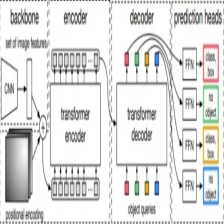
由上图可知，基于检测的追踪算法首先需要依赖于检测结果，这也就意味着我们可以使用任意的检测方法来与Sort方法进行组合，如YOLO+Sort、DETR+Sort等，在本章，我们首先使用YOLOv8+Sort方法来看一下这个目标追踪到底是如何实现的：

根据上面的Sort流程图，我们可以很明确我们的任务组成，即使用yolov8 进行目标检测、使用匈牙利算法对目标进行关联、使用卡尔曼滤波器对跟踪目标进行修正。

YOLOv8目标检测

为了使模型摆脱结构文件，我们使用导出的onnx模型文件进行目标检测，关于YOLOv8实现目标检测，博主在先前的博文中已经做了详细的介绍，这里博主给出一些关键代码：

首先是定义一个通用YOLO模型，这里面不定义模型结构，只定义一些模型所需的方法，如后处理方法、参数加载方法等

import time
import cv2
import numpy as np
import onnxruntime

from utils import xywh2xyxy, multiclass_nms,detections_dog

class YOLODet:
    #初始化YOLO模型
    def __init__(self, path, conf_thres=0.7, iou_thres=0.5):
        self.conf_threshold = conf_thres
        self.iou_threshold = iou_thres

        # Initialize model
        self.initialize_model(path)
    #调用推理
    def __call__(self, image):
        return self.detect_objects(image)
    #加载模型并获取模型的输入与输出结构
    def initialize_model(self, path):
        self.session = onnxruntime.InferenceSession(path,providers=onnxruntime.get_available_providers())
        # Get model info
        self.get_input_details()
        self.get_output_details()

    #执行模型推理过程
    def detect_objects(self, image):
        input_tensor = self.prepare_input(image)

        # Perform inference on the image
        outputs = self.inference(input_tensor)

        self.boxes, self.scores, self.class_ids = self.process_output(outputs)

        return self.boxes, self.scores, self.class_ids
    #前处理操作
    def prepare_input(self, image):
        self.img_height, self.img_width = image.shape[:2]

        input_img = cv2.cvtColor(image, cv2.COLOR_BGR2RGB)

        # Resize input image
        input_img = cv2.resize(input_img, (self.input_width, self.input_height))

        # Scale input pixel values to 0 to 1
        input_img = input_img / 255.0
        input_img = input_img.transpose(2, 0, 1)
        input_tensor = input_img[np.newaxis, :, :, :].astype(np.float32)

        return input_tensor

    #具体使用onnx推理
    def inference(self, input_tensor):
        start = time.perf_counter()
        outputs = self.session.run(self.output_names, {self.input_names[0]: input_tensor})

        # print(f"Inference time: {(time.perf_counter() - start)*1000:.2f} ms")
        return outputs
    #后处理操作
    def process_output(self, output):
        predictions = np.squeeze(output[0]).T

        # Filter out object confidence scores below threshold
        scores = np.max(predictions[:, 4:], axis=1)
        predictions = predictions[scores > self.conf_threshold, :]
        scores = scores[scores > self.conf_threshold]

        if len(scores) == 0:
            return [], [], []

        # Get the class with the highest confidence
        class_ids = np.argmax(predictions[:, 4:], axis=1)

        # Get bounding boxes for each object
        boxes = self.extract_boxes(predictions)

        # Apply non-maxima suppression to suppress weak, overlapping bounding boxes
        # indices = nms(boxes, scores, self.iou_threshold)
        indices = multiclass_nms(boxes, scores, class_ids, self.iou_threshold)

        return boxes[indices], scores[indices], class_ids[indices]
    #box转换，包含尺度变换与xywh转换
    def extract_boxes(self, predictions):
        # Extract boxes from predictions
        boxes = predictions[:, :4]

        # Scale boxes to original image dimensions
        boxes = self.rescale_boxes(boxes)

        # Convert boxes to xyxy format
        boxes = xywh2xyxy(boxes)

        return boxes
    #尺度变换
    def rescale_boxes(self, boxes):

        # Rescale boxes to original image dimensions
        input_shape = np.array([self.input_width, self.input_height, self.input_width, self.input_height])
        boxes = np.divide(boxes, input_shape, dtype=np.float32)
        boxes *= np.array([self.img_width, self.img_height, self.img_width, self.img_height])
        return boxes
    #画图
    def draw_detections(self, image, draw_scores=True, mask_alpha=0.4):

        return detections_dog(image, self.boxes, self.scores,
                              self.class_ids, mask_alpha)

    def get_input_details(self):
        model_inputs = self.session.get_inputs()
        self.input_names = [model_inputs[i].name for i in range(len(model_inputs))]

        self.input_shape = model_inputs[0].shape
        self.input_height = self.input_shape[2]
        self.input_width = self.input_shape[3]

    def get_output_details(self):
        model_outputs = self.session.get_outputs()
        self.output_names = [model_outputs[i].name for i in range(len(model_outputs))]

这个模型方法中的还需要一些方法，定义在util.py中，这是一个工具包，包含NMS操作、画图，IOU计算等方法

import numpy as np
import cv2

class_names = ['person', 'bicycle', 'car', 'motorcycle', 'airplane', 'bus', 'train', 'truck', 'boat', 'traffic light',
               'fire hydrant', 'stop sign', 'parking meter', 'bench', 'bird', 'cat', 'dog', 'horse', 'sheep', 'cow',
               'elephant', 'bear', 'zebra', 'giraffe', 'backpack', 'umbrella', 'handbag', 'tie', 'suitcase', 'frisbee',
               'skis', 'snowboard', 'sports ball', 'kite', 'baseball bat', 'baseball glove', 'skateboard', 'surfboard',
               'tennis racket', 'bottle', 'wine glass', 'cup', 'fork', 'knife', 'spoon', 'bowl', 'banana', 'apple',
               'sandwich', 'orange', 'broccoli', 'carrot', 'hot dog', 'pizza', 'donut', 'cake', 'chair', 'couch',
               'potted plant', 'bed', 'dining table', 'toilet', 'tv', 'laptop', 'mouse', 'remote', 'keyboard',
               'cell phone', 'microwave', 'oven', 'toaster', 'sink', 'refrigerator', 'book', 'clock', 'vase',
               'scissors', 'teddy bear', 'hair drier', 'toothbrush']


# Create a list of colors for each class where each color is a tuple of 3 integer values
rng = np.random.default_rng(3)
colors = rng.uniform(0, 255, size=(len(class_names), 3))


def nms(boxes, scores, iou_threshold):
    # Sort by score
    sorted_indices = np.argsort(scores)[::-1]

    keep_boxes = []
    while sorted_indices.size > 0:
        # Pick the last box
        box_id = sorted_indices[0]
        keep_boxes.append(box_id)

        # Compute IoU of the picked box with the rest
        ious = compute_iou(boxes[box_id, :], boxes[sorted_indices[1:], :])

        # Remove boxes with IoU over the threshold
        keep_indices = np.where(ious < iou_threshold)[0]

        # print(keep_indices.shape, sorted_indices.shape)
        sorted_indices = sorted_indices[keep_indices+1]

    return keep_boxes

def multiclass_nms(boxes, scores, class_ids, iou_threshold):

    unique_class_ids = np.unique(class_ids)

    keep_boxes = []
    for class_id in unique_class_ids:
        class_indices = np.where(class_ids == class_id)[0]
        class_boxes = boxes[class_indices,:]
        class_scores = scores[class_indices]

        class_keep_boxes = nms(class_boxes, class_scores, iou_threshold)
        keep_boxes.extend(class_indices[class_keep_boxes])

    return keep_boxes

def compute_iou(box, boxes):
    # Compute xmin, ymin, xmax, ymax for both boxes
    xmin = np.maximum(box[0], boxes[:, 0])
    ymin = np.maximum(box[1], boxes[:, 1])
    xmax = np.minimum(box[2], boxes[:, 2])
    ymax = np.minimum(box[3], boxes[:, 3])

    # Compute intersection area
    intersection_area = np.maximum(0, xmax - xmin) * np.maximum(0, ymax - ymin)

    # Compute union area
    box_area = (box[2] - box[0]) * (box[3] - box[1])
    boxes_area = (boxes[:, 2] - boxes[:, 0]) * (boxes[:, 3] - boxes[:, 1])
    union_area = box_area + boxes_area - intersection_area

    # Compute IoU
    iou = intersection_area / union_area

    return iou


def xywh2xyxy(x):
    # Convert bounding box (x, y, w, h) to bounding box (x1, y1, x2, y2)
    y = np.copy(x)
    y[..., 0] = x[..., 0] - x[..., 2] / 2
    y[..., 1] = x[..., 1] - x[..., 3] / 2
    y[..., 2] = x[..., 0] + x[..., 2] / 2
    y[..., 3] = x[..., 1] + x[..., 3] / 2
    return y


def draw_detections(image, boxes, scores, class_ids, mask_alpha=0.3):
    det_img = image.copy()

    img_height, img_width = image.shape[:2]
    font_size = min([img_height, img_width]) * 0.0006
    text_thickness = int(min([img_height, img_width]) * 0.001)

    det_img = draw_masks(det_img, boxes, class_ids, mask_alpha)

    # Draw bounding boxes and labels of detections
    for class_id, box, score in zip(class_ids, boxes, scores):
        color = colors[class_id]

        draw_box(det_img, box, color)

        label = class_names[class_id]
        caption = f'{label} {int(score * 100)}%'
        draw_text(det_img, caption, box, color, font_size, text_thickness)

    return det_img

def detections_dog(image, boxes, scores, class_ids, mask_alpha=0.3):
    det_img = image.copy()

    img_height, img_width = image.shape[:2]
    font_size = min([img_height, img_width]) * 0.0006
    text_thickness = int(min([img_height, img_width]) * 0.001)

    # det_img = draw_masks(det_img, boxes, class_ids, mask_alpha)

    # Draw bounding boxes and labels of detections

    for class_id, box, score in zip(class_ids, boxes, scores):

        color = colors[class_id]

        draw_box(det_img, box, color)
        label = class_names[class_id]
        caption = f'{label} {int(score * 100)}%'
        draw_text(det_img, caption, box, color, font_size, text_thickness)

    return det_img

def draw_box( image: np.ndarray, box: np.ndarray, color = (0, 0, 255),thickness: int = 2) -> np.ndarray:
    x1, y1, x2, y2 = box.astype(int)
    return cv2.rectangle(image, (x1, y1), (x2, y2), color, thickness)


def draw_text(image: np.ndarray, text: str, box: np.ndarray, color = (0, 0, 255),
              font_size: float = 0.001, text_thickness: int = 2) -> np.ndarray:
    x1, y1, x2, y2 = box.astype(int)
    (tw, th), _ = cv2.getTextSize(text=text, fontFace=cv2.FONT_HERSHEY_SIMPLEX,
                                  fontScale=font_size, thickness=text_thickness)
    th = int(th * 1.2)

    cv2.rectangle(image, (x1, y1),
                  (x1 + tw, y1 - th), color, -1)

    return cv2.putText(image, text, (x1, y1), cv2.FONT_HERSHEY_SIMPLEX, font_size, (255, 255, 255), text_thickness, cv2.LINE_AA)

def draw_masks(image: np.ndarray, boxes: np.ndarray, classes: np.ndarray, mask_alpha: float = 0.3) -> np.ndarray:
    mask_img = image.copy()

    # Draw bounding boxes and labels of detections
    for box, class_id in zip(boxes, classes):
        color = colors[class_id]

        x1, y1, x2, y2 = box.astype(int)

        # Draw fill rectangle in mask image
        cv2.rectangle(mask_img, (x1, y1), (x2, y2), color, -1)

    return cv2.addWeighted(mask_img, mask_alpha, image, 1 - mask_alpha, 0)

至此，YOLOv8目标检测便完成了，我们简单调用一下：

	model = 'yolov8n.onnx'
    base_conf,base_iou=0.5,0.3
    yolo_det = YOLODet.YOLODet(model, conf_thres=base_conf, iou_thres= base_iou)
    yolo_det = YOLODet.YOLODet(model, conf_thres=conf_thres, iou_thres= iou_thres)
    yolo_det(cv_src)
    cv_dst = yolo_det.draw_detections(cv_src)

匈牙利算法

匈牙利算法 (Hungarian Algorithm) 与 KM 算法 (Kuhn-Munkres Algorithm) 是用来解决多目标跟踪中的数据关联问题，匈牙利算法与 KM 算法都是为了求解二分图的最大匹配问题。

那什么是二分图呢？就是能分成两组 U 和 V ，其中， U 上的点不能相互连通，只能连接 V 中的点，同理， V 中的点不能相互连通，只能连去 U 中的点，这就是做二分图。

可以把二分图理解为视频中连续两帧中的所有检测框，第一帧所有检测框的集合称为 U ，第二帧所有检测框的集合称为 V 。同一帧的不同检测框不会为同一个目标，所以不需要互相关联，相邻两帧的检测框需要相互联通，最终将相邻两帧的检测框尽量完美地两两匹配起来。而求解这个问题的最优解就要用到匈牙利算法或者 KM 算法。

匈牙利算法和 KM 算法的原理这里就不在赘述了，相关的资料网上多的是，这里我们只需要知道他们是干什么的就可以了。其中 KM 算法是匈牙利算法的改进版本，它解决的是带权二分图的最优匹配问题。在多目标跟踪中目标关联是根据前一帧数据与后一帧数据的 IOU 作为权值进行关联的。

在 scipy 包中，通过 linear_sum_assignment 函数实现 KM 算法。

在Sort方法中，我们只需要调用即可

def linear_assignment(cost_matrix):
    x, y = linear_sum_assignment(cost_matrix)
    return np.array(list(zip(x, y)))

为什么使用卡尔曼滤波？

卡尔曼滤波无论是在单目标还是多目标领域都是很常用的一种算法，我们将卡尔曼滤波看做一种运动模型，用来对目标的位置进行预测，并且利用预测结果对跟踪的目标进行修正，属于自动控制理论中的一种方法。

那么，为什么要使用卡尔曼滤波来预测呢，我们直接使用原本的IOU追踪不可以吗？原因如下：

1. 在对视频中的目标进行跟踪时，当目标运动速度较慢时，很容易将前后两帧的目标进行关联，此时我们仅使用IOU追踪是可以的。(IOU追踪本质是计算上一帧与下一帧中目标的面积重合程度，进而将上一帧的检测目标与下一帧的检测目标联系在一起）
2. 但如果目标运动速度比较快，或者进行隔帧检测时，在后续帧中，目标A已运动到前一帧B所在的位置，而计算IOU实际上是计算其目标框的重合程度，这时再使用IOU进行关联就会得到错误的结果，将 A’与 B 关联在一起。

那怎么才能避免这种出现关联误差呢？我们可以在进行目标关联之前，对目标在后续帧中出现的位置进行预测，然后与预测结果进行对比关联:

我们在对比关联之前，先预测出 A 和 B 在下一帧中的位置，然后再使用实际的检测位置与预测的位置进行对比关联，只要预测足够精确，几乎不会出现由于速度太快而关联错误的情况。

卡尔曼滤波就是用来预测目标在后续帧中出现的位置。卡尔曼滤波器最大的优点是采用递归的方法来解决线性滤波的问题，它只需要当前的测量值和前一个周期的预测值就能够进行状态估计。由于这种递归方法不需要大量的存储空间，每一步的计算量小，计算步骤清晰，非常适合计算机处理，因此卡尔曼滤波受到了普遍的欢迎，在各种领域具有广泛的应用前景。

简单理解卡尔曼滤波分为两步，预测和更新。预测是根据上一周期的预测值对当前状进行估计。更新是用当前的观测值更新卡尔曼滤波器，用于下次状态的估计，这实际上就是递归。更新阶段是卡尔曼滤波的数据融合，它融合了估计值和观测值的结果，充分利用两者的不确定性来得到更加准确的估计。

以上就是卡尔曼滤波的简单思想，如果想了解详细的推理过程可以自行搜集资料进行研究，我们在这里只是了解其是如何实现预测并完成跟踪的。

卡尔曼滤波原理

卡尔曼滤波器的实现在 filterpy 包里。 filterpy 是一个实现了各种滤波器的 Python 模块，它实现著名的卡尔曼滤波和粒子滤波器。我们可以直接调用该库完成卡尔曼滤波器实现。

卡尔曼滤波的初始化如下：

class KalmanBoxTracker(object):
    """
    This class represents the internal state of individual tracked objects observed as bbox.
    """
    count = 0
    def __init__(self,bbox):
        #define constant velocity model
        self.kf = KalmanFilter(dim_x=7, dim_z=4)
        self.kf.F = np.array([[1,0,0,0,1,0,0],[0,1,0,0,0,1,0],[0,0,1,0,0,0,1],[0,0,0,1,0,0,0],[0,0,0,0,1,0,0],[0,0,0,0,0,1,0],[0,0,0,0,0,0,1]])
        self.kf.H = np.array([[1,0,0,0,0,0,0],[0,1,0,0,0,0,0],[0,0,1,0,0,0,0],[0,0,0,1,0,0,0]])
        self.kf.R[2:,2:] *= 10.
        self.kf.P[4:,4:] *= 1000. #give high uncertainty to the unobservable initial velocities
        self.kf.P *= 10.
        self.kf.Q[-1,-1] *= 0.01
        self.kf.Q[4:,4:] *= 0.01
        self.kf.x[:4] = convert_bbox_to_z(bbox)
        self.time_since_update = 0
        self.id = KalmanBoxTracker.count
        KalmanBoxTracker.count += 1
        self.history = []
        self.hits = 0
        self.hit_streak = 0
        self.age = 0

卡尔曼滤波实现：

（1）初始化：卡尔曼滤波器的状态变量和观测输入；
（2）跟踪器列表中目标框的预测；
（3）对于匹配上的目标框用检测框更新（并非直接替换）。

如下图所示，蓝色的分布是卡尔曼滤波预测值，棕色的分布是传感器的测量值，灰色的分布就是预测值基于测量值更新后的最优估计。

因此，要想获取其分布，我们在目标跟踪中，需要估计track的以下两个状态：

均值(Mean)	表示目标的位置信息，由bbox的中心坐标 (cx, cy)，宽高比r，高h，以及各自的速度变化值组成，由8维向量表示为 x = [cx, cy, r, h, vx, vy, vr, vh]，各个速度值初始化为0。
协方差(Covariance )	表示目标位置信息的不确定性，由8x8的对角矩阵表示，矩阵中数字越大则表明不确定性越大，可以以任意值初始化。

初始化卡尔曼滤波器

滤波器的状态变量x（7维）（在Sort中是7维，而在DeepSort中是8维）和观测输入z（4维）：

前四维分别表示目标框中心位置的x,y坐标，面积s和当前目标框的长宽比（即为观测输入，通过实参传入），最后三维则是横向，纵向，面积的变化速率，其中变化速率初始化为0。

跟踪器列表中目标框的预测（卡尔曼滤波预测）

首先插入一个形象的例子，这样后面理解起来会容易点：

假如现在有一辆在路上做直线运动的小车，该小车在 t时刻的状态可以用一个向量来表示 ，其中pt表示当前的位置，vt表示该车当前的速度。当然，司机还可以踩油门或者刹车来给车一个加速度ut，ut相当于是一个对车的控制量。显然，如果司机既没有踩油门也没有踩刹车，那么ut就等于0，此时车就会做匀速直线运动。

如果已知上一时刻 t-1时小车的状态，现在来考虑当前时刻t 小车的状态，显然有：

从以上公式可以看出：输出变量pt和vt都是输入变量的线性组合，这也就是卡尔曼滤波器被称为线性滤波器的原因。

既然上述公式表征了一种线性关系，那么就可以用一个矩阵来表示：

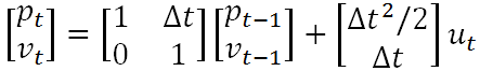
其中的分别就是状态转移矩阵F（表示如何从上一状态来推测当前状态）和控制矩阵B（表示控制量ut（加速度）如何作用于当前状态），至此就是卡尔曼滤波器的状态预测公式。

	在卡尔曼滤波器中状态转移矩阵F根据运动学公式可以确定为：这不是 对称矩阵
	F=（1000100,
        0100010,
        0010001,
        0001000,
        0000100,
        0000010,
        0000001）

在卡尔曼滤波器中运动形式（加速度）和状态转移矩阵的确定都是基于匀速运动模型(加速度为0），所以当前帧的状态可以如下表示：

其中，x' 是当前帧的状态变量，x 为上一帧的状态变量，实际上计算如下：

这时的状态是根据上一状态推测而来的，是一个估计值，应该对其进行修正以得到最优估计，那么就理应考虑到噪声的影响，若要引入噪声的影响，只要考虑噪声的方差σ即可，维度提高后，为了综合考虑各个维度偏离其均值的程度，需要引入协方差矩阵P。噪声同目标的状态一样也会进行传递，且预测模型本身并不是绝对准确的，用协方差矩阵 Q 来表示预测模型本身的噪声，那么所有噪声的传递可以表示如下（表示噪声在各个时刻间的传递关系）：

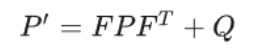
P为track在t-1时刻的协方差，Q为系统的噪声矩阵，代表整个系统的可靠程度，一般初始化为很小的值。

卡尔曼滤波更新

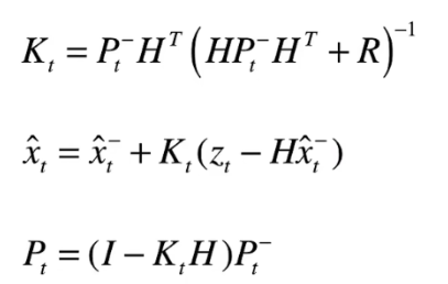
对于匹配上的目标框用检测框更新（并非直接替换）

先前我们说过，Sort算法中主要包含两个过程，分别是预测与更新，通过完成了预测过程，接下来，便是更新过程：

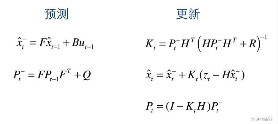
其中,首先要计算Kt，其表示卡尔曼增益，实际上是一种权重，由科学家推导所得，我们也就不要去纠结了，R代表检测误差

Zt代表检测结果

从目标的真实状态到我们看到的观测状态之间还有一个变换关系，这个变换关系叫做观测函数H，在卡尔曼滤波器中观测函数H可以确定为：

	H =（1000000,
         0100000,
         0010000,
         0001000）

Sort跟踪过程

了解了卡尔曼滤波与匈牙利算法后，我们接下来便是通过DeBug的方式来看看Sort到底是如何跟踪的。
首先，获得YOLO检测器的输出结果：

output= yolo_det(image)
outbox,score,cls=output

Sort跟踪算法中并不关心目标的类别，它只需要完成跟踪即可，所以只需要使用检测的目标框，将目标框传入Sort方法中，更新并获取轨迹

trackers = mot_tracker.update(outbox)

Sort方法中只有update这一个方法，用于更新并返回轨迹，代码如下：

class Sort(object):
    def __init__(self, max_age=1, min_hits=3, iou_threshold=0.3):
        """
        Sets key parameters for SORT
        """
        self.max_age = max_age #连续预测的最大次数，就是放在self.trackers跟踪器列表中的框用卡尔曼滤波器连续预测位置的最大次数
        self.min_hits = min_hits #最小更新的次数，就是放在self.trackers跟踪器列表中的框与检测框匹配上，
        # 然后调用卡尔曼滤波器类中的update函数的最小次数，min_hits不设置为0是因为第一次检测到的目标不用跟踪，
        # 只需要加入到跟踪器列表中，不会显示，这个值不能设大，一般就是1，表示如果连续两帧都检测到目标，
        self.iou_threshold = iou_threshold#IOU阈值
        self.trackers = []#存储追踪器
        self.frame_count = 0#读取的帧数量


    def update(self, dets=np.empty((0, 5))):
        """
        Params:
          dets - a numpy array of detections in the format [[x1,y1,x2,y2,score],[x1,y1,x2,y2,score],...]
        Requires: this method must be called once for each frame even with empty detections (use np.empty((0, 5)) for frames without detections).
        Returns the a similar array, where the last column is the object ID.
        NOTE: The number of objects returned may differ from the number of detections provided.
        """
        self.frame_count += 1
        # get predicted locations from existing trackers.
        trks = np.zeros((len(self.trackers), 5))
        ret = []
        for t, trk in enumerate(trks):
            pos = self.trackers[t].predict()[0]
            trk[:] = [pos[0], pos[1], pos[2], pos[3], 0]

        #numpy.ma.masked_invalid屏蔽出现无效值的数组（NaN或inf；numpy.ma.compress_rows压缩包含掩码值的2-D 数组的整行。
        trks = np.ma.compress_rows(np.ma.masked_invalid(trks))
        matched, unmatched_dets, unmatched_trks = associate_detections_to_tracks(dets, trks, self.iou_threshold)

        # update matched trackers with assigned detections
        for m in matched:
            self.trackers[m[1]].update(dets[m[0], :])

        # create and initialise new trackers for unmatched detections
        for i in unmatched_dets:
            trk = KalmanBoxTracker(dets[i,:])
            self.trackers.append(trk)
        i = len(self.trackers)

        #自后向前遍历，仅返回在当前帧出现且命中周期大于self.min_hits（除非跟踪刚开始）的跟踪结果；如果未命中时间大于self.max_age则删除跟踪器。
        for trk in reversed(self.trackers):
            d = trk.get_state()[0]
            if (trk.time_since_update < 1) and (trk.hit_streak >= self.min_hits or self.frame_count <= self.min_hits): #hit_streak：忽略目标初始的若干帧
                ret.append(np.concatenate((d,[trk.id+1])).reshape(1,-1)) # +1 as MOT benchmark requires positive
            i -= 1
            if(trk.time_since_update > self.max_age):
                self.trackers.pop(i)
        if(len(ret)>0):
            return np.concatenate(ret)
        return np.empty((0,5))

由于跟踪至少需要两帧数据（第一帧没法跟踪），我们先看第一帧的效果：

第一帧图像

matched, unmatched_dets, unmatched_trks = associate_detections_to_tracks(dets, trks, self.iou_threshold)

由于是第一帧，因此，只有unmacte_dets，即没匹配上的目标框，值为目标框的编号

没有与之匹配的轨迹，那么就创建，即初始化一个

for i in unmatched_dets:#第一帧时，没有匹配的轨迹，则创建对应的轨迹，一个一个的进行创建
       trk = KalmanBoxTracker(dets[i,:])
       self.trackers.append(trk)

利用检测框创建卡尔曼目标追踪器，在这个过程中会将检测结果由xyxy的形式转换为xyhr的形式（convert_bbox_to_z方法）

class KalmanBoxTracker(object):
    """
    This class represents the internal state of individual tracked objects observed as bbox.
    """
    count = 0
    def __init__(self,bbox):
        """
        Initialises a tracker using initial bounding box.
        """
        #define constant velocity model
        self.kf = KalmanFilter(dim_x=7, dim_z=4)
        self.kf.F = np.array([[1,0,0,0,1,0,0],[0,1,0,0,0,1,0],[0,0,1,0,0,0,1],[0,0,0,1,0,0,0],[0,0,0,0,1,0,0],[0,0,0,0,0,1,0],[0,0,0,0,0,0,1]])
        self.kf.H = np.array([[1,0,0,0,0,0,0],[0,1,0,0,0,0,0],[0,0,1,0,0,0,0],[0,0,0,1,0,0,0]])
        self.kf.R[2:,2:] *= 10.
        self.kf.P[4:,4:] *= 1000. #give high uncertainty to the unobservable initial velocities
        self.kf.P *= 10.
        self.kf.Q[-1,-1] *= 0.01
        self.kf.Q[4:,4:] *= 0.01
        self.kf.x[:4] = convert_bbox_to_z(bbox)
        self.time_since_update = 0
        self.id = KalmanBoxTracker.count
        KalmanBoxTracker.count += 1
        self.history = []
        self.hits = 0
        self.hit_streak = 0
        self.age = 0
  def convert_bbox_to_z(bbox):
    """
    Takes a bounding box in the form [x1,y1,x2,y2] and returns z in the form
      [x,y,s,r] where x,y is the centre of the box and s is the scale/area and r is
      the aspect ratio
    """
    w = bbox[2] - bbox[0]
    h = bbox[3] - bbox[1]
    x = bbox[0] + w/2.
    y = bbox[1] + h/2.
    s = w * h    #scale is just area
    r = w / float(h)
    return np.array([x, y, s, r]).reshape((4, 1))

随后，经过不断创建，得到了追踪器列表：

遍历跟踪器列表，判断当前的轨迹是否可用，若可用则添加到ret（结果）中，否则就删除该轨迹，最终返回结果

#自后向前遍历，仅返回在当前帧出现且命中周期大于self.min_hits（除非跟踪刚开始）的跟踪结果；如果未命中时间大于self.max_age则删除跟踪器。
        for trk in reversed(self.trackers):
            d = trk.get_state()[0]
            if (trk.time_since_update < 1) and (trk.hit_streak >= self.min_hits or self.frame_count <= self.min_hits): #hit_streak：忽略目标初始的若干帧
                ret.append(np.concatenate((d,[trk.id+1])).reshape(1,-1)) # +1 as MOT benchmark requires positive
                #这里的id加一是因为此处技术是从0开始的，在展示时要从1开始，即将xyxy与id合并加入到ret中
            i -= 1
            if(trk.time_since_update > self.max_age):#第一帧时不执行
                self.trackers.pop(i)
        if(len(ret)>0):
            return np.concatenate(ret)
        return np.empty((0,5))

trk.get_state方法是将轨迹中的（xyhr）的形式转换为检测中的（xyxy）的形式，因为这个数值是要展示的

def get_state(self):
        """
        Returns the current bounding box estimate.
        """
        return convert_x_to_bbox(self.kf.x)
def convert_x_to_bbox(x):
    """
    Takes a bounding box in the centre form [x,y,s,r] and returns it in the form
      [x1,y1,x2,y2] where x1,y1 is the top left and x2,y2 is the bottom right
    """
    #将[x,y,s,r]形式的bbox，转为[x1,y1,x2,y2]形式
    w = np.sqrt(x[2] * x[3])
    h = x[2] / w
    return np.array([x[0]-w/2.,x[1]-h/2.,x[0]+w/2.,x[1]+h/2.]).reshape((1,4))

至此，得到了第一帧图像的跟踪结果，即将检测结果作为轨迹结果展示。

第二帧图像

同样的，先获取第二帧图像中的目标：

output= yolo_det(image)
outbox,score,cls=output

这一帧图像中只有9个目标

再次进入跟踪器进行更新：

trks = np.zeros((len(self.trackers), 5))

由于trackers内有轨迹，故创建的trks如下：

预测位置

此时，要根据上一帧数据预测当前帧的目标位置：

for t, trk in enumerate(trks):#第一帧时，里面没有东西，直接跳过
            pos = self.trackers[t].predict()[0]
            trk[:] = [pos[0], pos[1], pos[2], pos[3], 0]

具体的，跟踪器的预测方法如下：

def predict(self):
        """
        Advances the state vector and returns the predicted bounding box estimate.
        """
        if(self.kf.x[6]+self.kf.x[2]<=0):
            self.kf.x[6] *= 0.0
        self.kf.predict()
        self.age += 1
        if(self.time_since_update>0):
            self.hit_streak = 0
        self.time_since_update += 1
        self.history.append(convert_x_to_bbox(self.kf.x))#记录历史坐标，这个坐标是预测的坐标
        return self.history[-1]#历史坐标的最后一个即当前的预测位置

卡尔曼滤波的预测方法如下：

def predict(self, u=None, B=None, F=None, Q=None):
        """
        Predict next state (prior) using the Kalman filter state propagation
        equations.

        Parameters
        ----------

        u : np.array
            Optional control vector. If not `None`, it is multiplied by B
            to create the control input into the system.

        B : np.array(dim_x, dim_z), or None
            Optional control transition matrix; a value of None
            will cause the filter to use `self.B`.

        F : np.array(dim_x, dim_x), or None
            Optional state transition matrix; a value of None
            will cause the filter to use `self.F`.

        Q : np.array(dim_x, dim_x), scalar, or None
            Optional process noise matrix; a value of None will cause the
            filter to use `self.Q`.
        """

        if B is None:
            B = self.B
        if F is None:
            F = self.F
        if Q is None:
            Q = self.Q
        elif isscalar(Q):
            Q = eye(self.dim_x) * Q

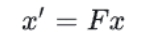
        # x = Fx + Bu
        if B is not None and u is not None:
            self.x = dot(F, self.x) + dot(B, u)#更新x即轨迹的目标信息
        else:
            self.x = dot(F, self.x)

        # P = FPF' + Q
        self.P = self._alpha_sq * dot(dot(F, self.P), F.T) + Q

        # save prior
        self.x_prior = self.x.copy()
        self.P_prior = self.P.copy()

此时，便会直接将数值更新，即根据上一帧的数值计算出当前帧的预测值。当前轨迹内的信息如下：

按照上面的值，我们看x，其后面3位为0，那么，事实上，这个所谓的预测值就是上一帧的位置，这其实与IOU匹配是一样的，但之所以卡尔曼滤波追踪能够取得较好的性能，是由于其预测与追踪的共同作用，即要不断使用后续的检测结果来修正预测结果，x的值在更新时再次改变，此时的预测值只不过是一个中间值罢了。通过这样不断的修正，预测值就会不断的去接近真正的下一帧的检测值了。

将预测的位置保存到trk中：

trk[:] = [pos[0], pos[1], pos[2], pos[3], 0]

此时的trk的值是xyxy的形式

匈牙利匹配

此时，trks中的数据为根据上一帧数据预测的数据（实际上就是上一帧的数据，这里是做区分）

接下来，便是进行预测框与当前帧检测框的匹配了，在第一帧时，由于没有先前的数据，所以也就无法匹配成功，我们看下第二帧的效果：

#传入的参数分别是上一帧的预测结果（trks)，当前帧的检测结果(dets)以及IOU阈值
matched, unmatched_dets, unmatched_trks = associate_detections_to_tracks(dets, trks, self.iou_threshold)

def associate_detections_to_tracks(detections,trackers,iou_threshold = 0.3):
    """
    Assigns detections to tracked object (both represented as bounding boxes)
    Returns 3 lists of matches, unmatched_detections and unmatched_trackers
    """
    if(len(trackers)==0):#如果没有轨迹的话，即第一帧的情况，直接返回空即可
        return np.empty((0,2),dtype=int), np.arange(len(detections)), np.empty((0,5),dtype=int)

    #计算两两间的交并比，调用linear_assignment进行匹配
    iou_matrix = iou_batch(detections, trackers)#计算IOU，并构造代价矩阵,iou_matrix为ndarry(9,10)
    
    if min(iou_matrix.shape) > 0:
        a = (iou_matrix > iou_threshold).astype(np.int32)#选出检测值与预测值的iou大于阈值的，a的维度也是（9，10）值为1或0
        if a.sum(1).max() == 1 and a.sum(0).max() == 1:#按行求和以及按列求和的值的max为1，说明每行每列只有一个符合的，此时不需要计算匹配了，直接用这个结果即可
            matched_indices = np.stack(np.where(a), axis=1)
        else:#否则，执行匈牙利匹配
            matched_indices = linear_assignment(-iou_matrix)#匈牙利匹配是按少的那个匹配，比如（9，10）则必定只能匹配成功9个，此时返回结果维度为（9，2）2代表的是匹配的id，其中第一个代表检测框id，第二个代表预测框id
    else:
        matched_indices = np.empty(shape=(0,2))

    #记录未匹配的检测框及轨迹
    unmatched_detections = []
    for d, det in enumerate(detections):#matched_indices中第一个为检测框编号
        if(d not in matched_indices[:,0]):
            unmatched_detections.append(d)
    unmatched_trackers = []
    for t, trk in enumerate(trackers):
        if(t not in matched_indices[:,1]):
            unmatched_trackers.append(t)

    #过滤掉IoU低的匹配
    matches = []#将已经匹配成功的中iou阈值较低的都去除，即把的对应的编号加入到对应的未匹配列表中，否则的话，这些就是要真正的匹配成功的轨迹与检测框了
    for m in matched_indices:#看看匈牙利匹配的结果中有没有低于阈值的
        if(iou_matrix[m[0], m[1]]<iou_threshold):
            unmatched_detections.append(m[0])
            unmatched_trackers.append(m[1])
        else:
            matches.append(m.reshape(1,2))
    if(len(matches)==0):
        matches = np.empty((0,2),dtype=int)
    else:
        matches = np.concatenate(matches,axis=0)

    return matches, np.array(unmatched_detections), np.array(unmatched_trackers)

该过程中一些重要的数据结果如下：

匈牙利匹配代价矩阵

匈牙利匹配结果，第一个为检测框id，第二个为预测框id

最终经过IOU阈值筛选后，得到的匹配的检测框与轨迹，可以看到，其有一组匹配失败了

未匹配上的检测框与轨迹，由于当前帧检测框有9个，上一帧的轨迹有10个，因此必定有一个未匹配的轨迹。

修正轨迹

将匹配成功的matched，未匹配的轨迹以及未匹配的检测框返回即可，随后根据当前帧的检测结果来对预测进行修正。

for m in matched:#如果有匹配上的则利用刚刚检测的结果来更新，即用于卡尔曼滤波预测，第一帧时不执行
            self.trackers[m[1]].update(dets[m[0], :])
            
def update(self,bbox):
        """
        Updates the state vector with observed bbox.
        """
        self.time_since_update = 0
        self.history = []#清空历史
        self.hits += 1
        self.hit_streak += 1
        self.kf.update(convert_bbox_to_z(bbox))#卡尔曼更新

卡尔曼更新操作如下，该方法也是封装好的，我们会用即可，执行的便是如下操作：

比如X的值先前如下：

更新完后的值如下，可以看到，其值发生了变化。

def update(self, z, R=None, H=None):
        """
        Add a new measurement (z) to the Kalman filter.

        If z is None, nothing is computed. However, x_post and P_post are
        updated with the prior (x_prior, P_prior), and self.z is set to None.

        Parameters
        ----------
        z : (dim_z, 1): array_like
            measurement for this update. z can be a scalar if dim_z is 1,
            otherwise it must be convertible to a column vector.

        R : np.array, scalar, or None
            Optionally provide R to override the measurement noise for this
            one call, otherwise  self.R will be used.

        H : np.array, or None
            Optionally provide H to override the measurement function for this
            one call, otherwise self.H will be used.
        """

        # set to None to force recompute
        self._log_likelihood = None
        self._likelihood = None
        self._mahalanobis = None

        if z is None:
            self.z = np.array([[None]*self.dim_z]).T
            self.x_post = self.x.copy()
            self.P_post = self.P.copy()
            self.y = zeros((self.dim_z, 1))
            return

        z = reshape_z(z, self.dim_z, self.x.ndim)

        if R is None:
            R = self.R
        elif isscalar(R):
            R = eye(self.dim_z) * R

        if H is None:
            H = self.H

        # y = z - Hx
        # error (residual) between measurement and prediction
        self.y = z - dot(H, self.x)

        # common subexpression for speed
        PHT = dot(self.P, H.T)

        # S = HPH' + R
        # project system uncertainty into measurement space
        self.S = dot(H, PHT) + R
        self.SI = self.inv(self.S)
        # K = PH'inv(S)
        # map system uncertainty into kalman gain
        self.K = dot(PHT, self.SI)

        # x = x + Ky
        # predict new x with residual scaled by the kalman gain
        self.x = self.x + dot(self.K, self.y)

        # P = (I-KH)P(I-KH)' + KRK'
        # This is more numerically stable
        # and works for non-optimal K vs the equation
        # P = (I-KH)P usually seen in the literature.

        I_KH = self._I - dot(self.K, H)
        self.P = dot(dot(I_KH, self.P), I_KH.T) + dot(dot(self.K, R), self.K.T)

        # save measurement and posterior state
        self.z = deepcopy(z)
        self.x_post = self.x.copy()
        self.P_post = self.P.copy()

利用当前帧的检测结果修正轨迹中的结果后，之后的过程便是与第一帧相同了，将轨迹添加到rets中，即完成了轨迹跟踪过程
目标跟踪的结果，是当前帧对上一帧预测结果修正后的结果，他并不是当前帧的检测结果，而是修正后的预测结果。

第三帧图像

由于第二帧与第一帧的作用，卡尔曼滤波器中的x值已经发生了变化

X的值先前如下：

更新完后的值如下，可以看到，其值发生了变化。

那么在进行预测时，上一帧的预测结果就不是当前帧的检测结果了，其会有些许变化，这也就是不断修正的过程，即随着更新越多，预测的也就精确。

至此，便完成了目标跟踪的Sort算法，最终，根据上述过程绘制了Sort算法的流程图：