TreeExplainer原文精读: 用于树的可解释人工智能SHAP Tree

TreeExplainer原文精读: 用于树的可解释AI

参考论文:

1. Lundberg, Scott M., et al. “From local explanations to global understanding with explainable AI for trees.” Nature machine intelligence 2.1 (2020): 56-67. https://www.nature.com/articles/s42256-019-0138-9
2. 博弈论与机器学习的碰撞 - 探究模型Shap值背后的秘密：https://zhuanlan.zhihu.com/p/356565166
3. SHAP：用博弈论大一统解释模型预测！A Unified Approach to Interpreting Model Predictions 引用破万：https://zhuanlan.zhihu.com/p/596538131
4. Understanding Shapley value explanation algorithms for trees：https://hughchen.github.io/its_blog/index.html#algorithm

1. Shapley values

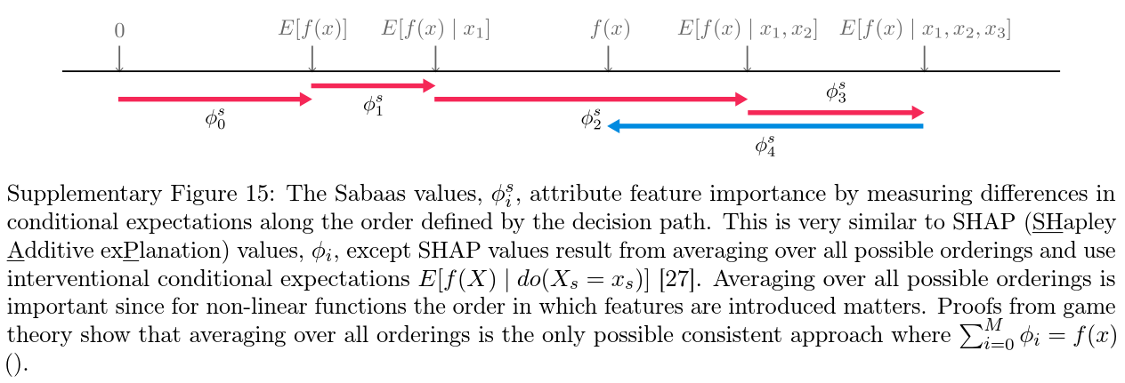
在这里，我们回顾了博弈论中Shapley值的唯一性保证，因为它们适用于机器学习模型预测的局部解释⁹。如本文所应用的，Shapley值是通过将每个特征一次一个地引入模型输出的条件期望函数$f_x(S)=E[f(X)|do(X_S=x_S)]$来计算的，并将每个步骤产生的变化归因于引入的特征；然后对所有可能的特征排序对该过程进行平均（补充图15）。注意，$S$是我们所依赖的特征集，$X$是表示模型$M$的输入特征的随机变量，$X$是当前预测的模型输入向量，并且我们遵循参考文献^[11]中建议的因果do-notation公式。这改进了原始SHAP特征扰动公式的动机。一种等效的配方是参考文献^[10]中讨论的随机基线方法。Shapley值代表了一类广泛的可加特征归因方法^[3]中唯一可能的方法，该方法将同时满足三个重要特性：局部准确性(local accuracy)、一致性(consistency)和缺失性(missingness)。

补充说明:

局部准确性(Local Accuracy)，缺失性(Missingness)，一致性(Consistency)实际上能够通过之前提到的shapley 四大性质(即可加性、对称性、空值性和线性)推出。

1. 局部准确性等同于可加性，含义是特征的shap值之和总是等于模型的实际输出。
2. 缺失性等同于Null Player性质，当一个特征对任意一个特征组合的增益均为0，则该特征贡献为0。
3. 一致性可由对称性，可加性，缺失性推出。它是指对于两个模型，如果一个特征对于模型A的任意特征组合的增益，均大于等于该特征对于模型B的任意特征组合的增益，那么该特征对模型A的贡献也大于等于对模型B的贡献。

1.1 Property 1 (local accuracy/efficiency).

局部精度（在博弈论中称为“效率”）表明，当对特定输入$x$近似原始模型$f$时，每个特征$i$的解释的归因值${\varphi }_i$应加起来为输出$f(x)$：
$$f(x)={\varphi }_0(f)+\sum _{i=1}^M{\varphi }_i(f,x)$$
特征属性的总和${\varphi }_i(f,x)$与原始模型输出$f(x)$相匹配，其中${\varphi }_0(f)=E[f(z)]=f_x(\Phi )$。

局部准确性的含义: 等同于可加性，特征的SHAP值之和总是等于模型的实际输出。

1.2 Property 2 (consistency/monotonicity).

一致性（博弈论中称为“单调性”）表明，如果模型发生变化，使得某些特征的贡献增加或保持不变，而不考虑其他输入，则该输入的贡献不应减少。

对于任意两个模型$f$和$f^{\prime }$, 如果
$$f_x^{\prime }(S)-f_x^{\prime }(S\backslash i)\ge f_x(S)-f_x(S\backslash i)$$
对于所有的特征子集$S\in \mathcal{F}$, 那么${\Phi }_i(f^{\prime },x)\ge {\Phi }_i(f,x)$。

一致性的含义: 对于两个模型，如果一个特征对于模型A的任意特征组合的增益，均大于等于该特征对于模型B的任意特征组合的增益，那么该特征对模型A的贡献也大于等于对模型B的贡献。

1.3 Property 3 (missingness).

缺失性（类似于博弈论中的“零效应”）要求对集合函数$f_x$没有影响的特征没有指定的影响。我们所知道的所有局部以前的方法都满足缺失性。

如果
$$f_x(S\bigcup i)=f_x(S)$$
对所有特征子集$S\in \mathcal{F}$, 有${\varphi }_i(f,x)=0$。

当一个特征对任意一个特征组合的增益均为0，则该特征贡献为0。

同时满足这些特性的唯一方法是使用经典的Shapley值。

1.4 定理1: Theorem 1

定理1的等价公式已经在参考文献^[3]中给出, 并且来自合作博弈论的结果^[36], 其中的值${\varphi }_i$被称为Shapley值^[9]。Shapley值的定义独立于用于测量一组特征的重要性的集合函数。由于这里我们使用的是$f_x$，这是模型输出的条件期望函数，所以我们计算的是更具体的SHAP值^[3，11]。有关这些值的更多属性，请参见补充方法5。

补充方法5：SHAP values的额外属性

除了正文中描述的三个性质外，SHAP值还满足先前提出的几种良好解释方法的性质：

• 实现不变性(Implementation invariance)，即模型的解释应仅取决于模型的行为，而不是如何实现[65]。这是一个理想的特性，因为如果两个模型在所有输入中表现相同，那么它们应该得到对其行为的相同解释，这是很自然的。SHAP值满足此属性，因为等式4仅取决于模型的行为，而不取决于任何实现细节。
• 线性(Linearity)，即通过在相同输入上线性组合其他两个模型而形成的联合模型应具有与每个组成模型的解释相同的线性组合的解释[64]。SHAP值遵循线性，因为这是Shapley值的一个众所周知的特性[58]。
• 敏感性-n(Sensitivity-n)，这是一个衡量标准，Shapley值提供了一个合理的（在某种意义上是最优的）解决方案[1]。敏感性-n衡量一组特征归属值能多好地代表掩盖n个随机特征集对模型输出的eff影响。对于复杂的函数，没有一种方法可以通过对特征归属值的求和来完美地表示所有的高阶effects，但是Shapley值提供了一种原则性的方法来挑选解决方案。这是因为Shapley值是唯一一个既一致（属性2），又局部准确（意味着当所有特征都包括在内时，数值与模型的输出相加）的解决方案。
• 解释的连续性(Explanation continuity)，这说明对于连续模型，输入的微小变化应该导致解释的微小变化[44]。SHAP值满足这一点，因为它们是模型输出的线性函数，因此，如果基础模型是连续的，SHAP值也将是连续的。 请注意，对于TreeExplainer，这一属性通常不适用，因为基于树的模型不是连续的。

**定理1.**只有一种基于$f_x$的可能特征贡献方法满足属性1、2和3：
$${\varphi }_i(f,x)=\sum _{R\in \mathcal{R}}\frac{1}{M!}[f_x(P_i^R\bigcup i)-f_x(P_i^R)]$$
其中，$\mathcal{R}$是所有特征排序的集合，$P_i^R$是在排序$R$中位于特征$i$之前的所有特征的集合，$M$是模型的输入特征数。

2. 具有路径依赖特征扰动的TreeExplainer

我们分三个阶段描述TreeExplainer背后的算法。首先，我们描述了使用路径依赖特征扰动的Tree SHAP算法的一个容易理解（但很慢）的版本（算法1），然后我们介绍了使用路径依赖的Tree SHAP的复杂多项式时间版本，最后我们描述了使用干预性（边缘）特征扰动的Tree SHAP算法（其中$f_x(S)$正好等于$E[f(X)\mid do(X_S=x_S)]$）。虽然求解Shapley值一般来说是NP-hard¹²，但这些算法表明，通过限制我们对树的关注，我们可以在低阶多项式运行时间内找到精确的解决方案。

使用路径特征依赖的Tree SHAP算法并不精确计算$E[f(X)\mid do(X_S=x_S)]$，而是使用算法1进行近似计算，该算法使用模型的覆盖信息，即哪些训练样本在树上走了哪些路径。这很方便，因为它意味着我们不需要提供背景数据集来解释模型（算法1也直接与经典的 "增益 "式特征重要性所使用的遍历相似）。

鉴于$f_x$是用算法1定义的，Tree SHAP路径依赖就可以精确地计算出方程(4)。假设$T$是树的数量，$D$是任何树的最大深度，$L$是叶子的数量，Tree SHAP路径依赖的最坏情况下的复杂度是$O(TL{D}^2)$。这代表了比以前的精确Shapley方法的指数级复杂度的改进，后者的复杂度为$O(TLM{2}^M)$，其中$M$是输入特征的数量。

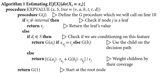
如果我们忽略计算的复杂性，那么我们可以通过计算$f_x(S)$，然后直接使用方程$(4)$来计算树的SHAP值。 算法1计算$f_x(S)$，其中树包含树的信息。 $v$是一个节点值的向量；对于内部节点，我们分配的是内部值。向量$a$和$b$代表每个内部节点的左和右节点索引。向量$t$包含每个内部节点的阈值，$d$是内部节点中用于分割的特征的索引向量。向量$r$代表每个节点的覆盖率（即有多少数据样本落在该子树中）。

2.1 算法1： Estimating E[f(X)|do(XS = xS)]

算法1估计$E[f(X)\mid do(XS=xS)]$的方法是，如果分割特征在$S$中，则递归遵循$x$的决策路径，如果分割特征不在$S$中，则取两个分支的加权平均数。算法1的计算复杂性与树中的叶子数量成正比，当用于一个集成分类器中的所有$T$树并插入公式$(4)$时，计算所有$M$个特征的SHAP值的复杂性为$O(TLM{2}^M)$。

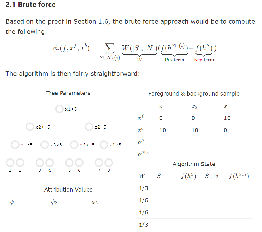
如何理解算法1？==> 代码中是如何体现的？

参考: https://hughchen.github.io/its_blog/index.html#brute_force

def ite_brute(array xf, array xb, tree T, array N):
   phi = [0]*len(xf)
   ##对于特征集合中的每个特征。
   for each feature i in N:  
       ##对于N个特征中除去特征i的集合，计算该集合的幂集(即由该集合全部子集为元素构成的集合)。
       for each set S in powerset(setminus(N,i)):
           hs  = [xf[j] for j in N if j in S else xb[j]] # Hybrid samples
           hsi = [xf[j] for j in N if j in union(S,i) else xb[j]]
           fxs  = T.predict(hs) # Predictions
           fxsi = T.predict(hsi)
           W = (len(S)!*(len(N)-len(S)-1)!)/(len(N)!) # Weight
           phi[i] += W*(fxsi-fxs) # Calculate phi contributi

蛮力算法的复杂度为：O(d×(tree depth)×2d)

2.2 使用路径依赖的Tree SHAP的复杂多项式时间版本

现在，我们计算出与上述相同的数值，但在多项式时间而不是指数时间内。具体来说，我们提出了一种在$O(TL{D}^2)$时间和$O(D^2+M)$内存中运行的算法，其中对于平衡树来说，深度变成了$D=logL$。 回顾一下，$T$是树的数量，$L$是任何树中叶子的最大数量，$M$是特征的数量。

多项式时间算法的直觉是递归地跟踪所有可能的子集有多大比例流向树的每个叶子。这类似于对方程（4）中所有$2^M$个子集$S$同时运行算法1。请注意，一个子集$S$可以落入多个叶子。简单地跟踪有多少个子集（由第9行的算法1的盖子分割加权）从树的每个分支通过似乎是合理的。然而，这结合了不同大小的子集，因此无法对这些子集进行适当的加权，因为公式（4）中的权重取决于$\mid S\mid$。为了解决这个问题，我们在递归过程中跟踪每个可能的子集大小，而不仅仅是对所有子集进行单一的计数。算法2中的EXTEND方法根据一个给定的1和0的分数来增长所有这些子集的大小，而UNWIND方法则反转这个过程，并与EXTEND进行交换。EXTEND方法是在我们下降树的过程中使用的。UNWIND方法用于当我们在同一特征上分裂两次时撤销之前的扩展，并撤销叶子内部路径的每一次扩展，以计算路径中每个特征的权重。 请注意，EXTEND在递归过程中不仅跟踪子集的比例，而且还跟踪方程（4）中应用于这些子集的权重。由于方程（4）中应用于子集的权重在包括特征$i$时是不同的，所以一旦我们在一个叶子中着陆，我们需要分别UNWIND每个特征的权重，以计算每个特征的SHAP值在该叶子中的正确权重。只在叶子中进行 UNWIND 的能力取决于 UNWIND 和 EXTEND 的换算性质。

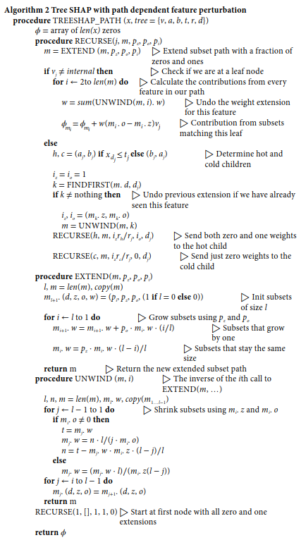
在算法2中，$m$是我们到目前为止所分割的唯一特征的路径，包含四个属性：(1) $d$，特征索引；(2)$ z$，流经该分支的"zero"路径（该特征不在集合$S$中）的比例；(3) $o$，流经该分支的 "one "路径（该特征在集合S中）的比例；以及(4)$w$，用于保存给定cardinality(基数)的集合的比例，以其Shapley加权(公式(4))。请注意，$w$所捕获的权重不需要考虑在决策路径上尚未看到的特征，所以方程$(4)$中的$M$的有效大小是随着我们下降树而增长的。我们使用**点符号(dot notation)**来访问成员值，对于整个向量$m\cdot d$表示所有特征索引的向量。值$p_z$、$p_o$和$p_i$代表要扩展子集的zeros和ones的比例，以及用于进行最后一次分割的特征的索引。我们对树和输入向量$x$使用与算法1相同的符号。当给定输入x时，树所跟随的子节点称为 "hot"子节点。请注意，算法2（在开源代码中实现）的正确性已经得到验证，它与基于算法1的蛮力方法进行了比较，适用于成千上万的随机模型和$M<15$的数据集。

问题：为什么要求特征数目小于15？如何理解呢？

Figure 8: Naive algorithm for the tree and samples specified in Figure 5.

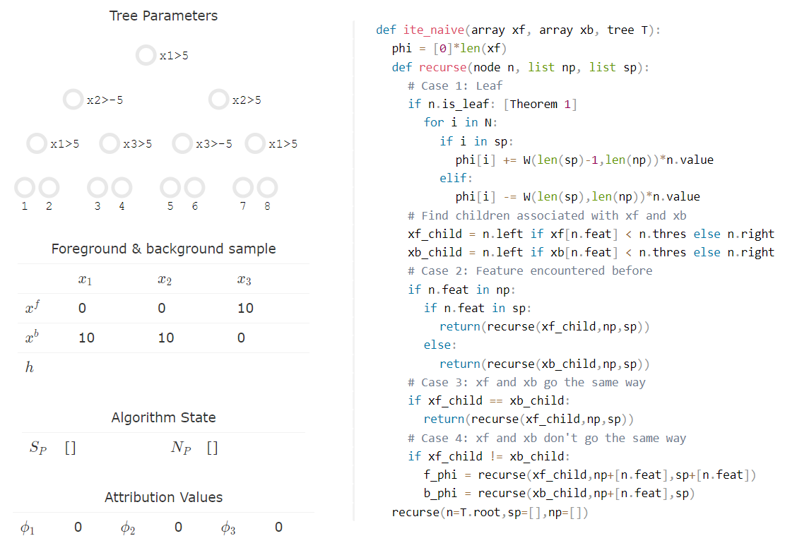
def ite_naive(array xf, array xb, tree T):
    phi = [0]*len(xf)
    def recurse(node n, list np, list sp):
        # Case 1: Leaf
        if n.is_leaf: [Theorem 1]
        	for i in N:
        		if i in sp:
        			phi[i] += W(len(sp)-1,len(np))*n.value
        		elif:
        			phi[i] -= W(len(sp),len(np))*n.value
        # Find children associated with xf and xb
        xf_child = n.left if xf[n.feat] < n.thres else n.right
        xb_child = n.left if xb[n.feat] < n.thres else n.right
        # Case 2: Feature encountered before
        if n.feat in np:
            if n.feat in sp:
                return(recurse(xf_child,np,sp))
            else:
                return(recurse(xb_child,np,sp))
        # Case 3: xf and xb go the same way
        if xf_child == xb_child:
            return(recurse(xf_child,np,sp))
        # Case 4: xf and xb don't go the same way
        if xf_child != xb_child:
            f_phi = recurse(xf_child,np+[n.feat],sp+[n.feat])
            b_phi = recurse(xb_child,np+[n.feat],sp)
    recurse(n=T.root,sp=[],np=[])

2.3 复杂性分析(Complexity analysis)

算法2将树和树之和的精确SHAP值计算复杂性从指数级降低到低阶多项式（因为两个函数之和的SHAP值是原始函数的SHAP值之和）。第6、12、21、27和34行的循环都以子集路径$m$的长度为界，它以$D$为界，即最大的树的深度。这意味着UNWIND和EXTEND的复杂度是以O(D)为界限的。对RECURSE的每次调用对内部节点产生O(D)的复杂性，或者对叶子节点产生$O(D^2)$的复杂性，因为UNWIND被嵌套在一个以D为界限的循环中。对于一个由T个树组成的整体，这个约束变成了$O(TL{D}^2)$。如果我们假设这些树是平衡的，那么$D=logL$，这个界限就变成了$O(TLlo{g}^{2}L)$。

3. 具有干预性特征扰动的TreeExplainer。

带有干预性特征扰动的TreeExplainer(正是方程(4))可以以最坏情况下的复杂度$O(TLDN)$计算，其中N是用于条件期望的背景样本数。

Tree SHAP算法为树和树的总和提供了快速的精确解(因为Shapley值的线性⁹)，但有些时候，不仅要解释树的直接输出，还要解释树的输出的非线性变换，这是非常有用的。一个引人注目的例子是解释一个模型的损失函数，这对模型的监测和调试非常有用。不幸的是，没有简单的方法来调整一个函数的Shapley值，以准确考虑模型输出的非线性转换。相反，我们将以前提出的组合式近似法(Deep SHAP)^[3]与Tree SHAP的思想结合起来，创造了一种专门针对树的快速方法。组合式方法需要对用于计算期望值的数据集中的每个背景样本进行迭代，因此我们设计了算法3来单独循环处理背景样本。

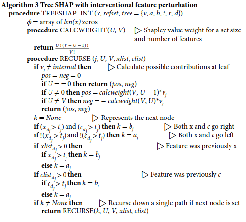
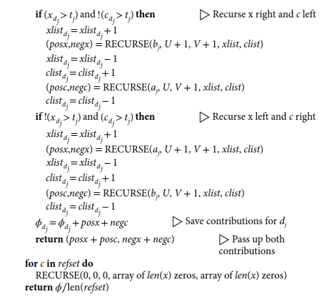
3.1 算法3：具有干预性特征扰动的Tree SHAP

**Interventional Tree SHAP(通过因果律)**在条件集$S$和其余特征集$(x_S\perp x_S)$之间强制执行了一种独立性。 利用这种独立性，关于$R$个单独的背景样本的Shapley值可以被平均到一起，以获得完整分布的属性。因此，算法3是通过在一棵树上遍历由单个前景和背景样本组成的混合路径来进行的。在每个内部节点，RECURSE向下遍历树，保持本地状态以跟踪上游特征集，以及所分割的特征是来自前景还是背景样本。然后，在每个叶子上，计算出两个贡献–一个是正贡献，一个是负贡献。每个叶子的正负贡献都取决于被解释的特征。然而，通过在每一片叶子上迭代所有的特征来计算Shapley值会导致一个二次方的时间算法。相反，RECURSE将这些贡献传递给父节点，并根据前景和背景样本穿越的方向，决定是将正贡献还是负贡献分配给被分割的特征。然后，内部节点将两个正贡献汇总为一个正贡献，将两个负贡献汇总为一个负贡献，并将其传递给其父节点。

请注意，每个叶子的正贡献和负贡献都是两个变量的函数：(1)$U$，沿路与前景样本相匹配的特征数量；（2）$V$，沿路遇到的独特特征总数。这意味着，对于不同的叶子，将考虑不同的特征总数$V$。这使得算法只考虑$O(L)$项，而不是指数级的项。 尽管在每个叶子上有不同的$U$，但干预Tree SHAP完全可以计算出传统的Shapley值公式（对于任何给定的路径，它考虑的是固定的特征总数$\ge V$），因为求和中的项很好地组合在一起。

Figure 10: Dynamic programming algorithm for the tree and samples specified in Figure 5.

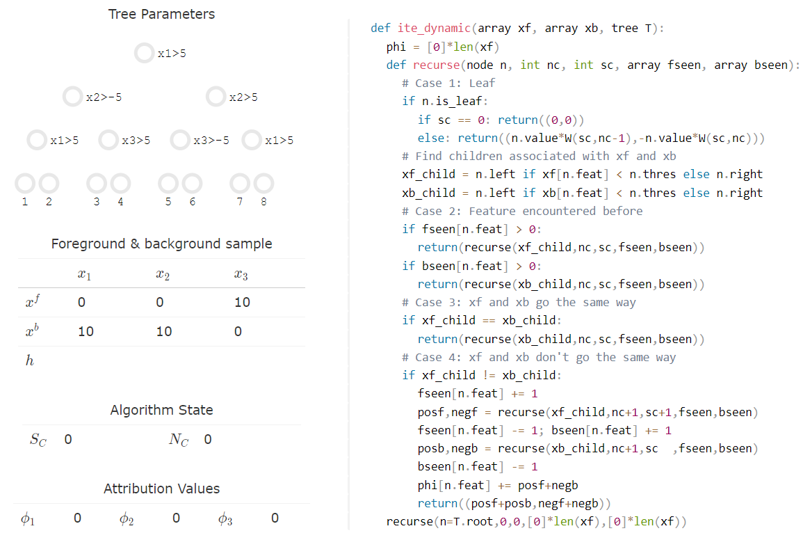
def ite_dynamic(array xf, array xb, tree T):
    phi = [0]*len(xf)
    def recurse(node n, int nc, int sc, array fseen, array bseen):
        # Case 1: Leaf
        if n.is_leaf:
            if sc == 0: return((0,0))
            else: return((n.value*W(sc,nc-1),-n.value*W(sc,nc)))
        # Find children associated with xf and xb
        xf_child = n.left if xf[n.feat] < n.thres else n.right
        xb_child = n.left if xb[n.feat] < n.thres else n.right
        # Case 2: Feature encountered before
        if fseen[n.feat] > 0:
            return(recurse(xf_child,nc,sc,fseen,bseen))
        if bseen[n.feat] > 0:
            return(recurse(xb_child,nc,sc,fseen,bseen))
        # Case 3: xf and xb go the same way
        if xf_child == xb_child:
        	return(recurse(xb_child,nc,sc,fseen,bseen))
        # Case 4: xf and xb don't go the same way
        if xf_child != xb_child:
        	fseen[n.feat] += 1
            posf,negf = recurse(xf_child,nc+1,sc+1,fseen,bseen)
            fseen[n.feat] -= 1; bseen[n.feat] += 1
            posb,negb = recurse(xb_child,nc+1,sc  ,fseen,bseen)
            bseen[n.feat] -= 1
            phi[n.feat] += posf+negb
            return((posf+posb,negf+negb))
    recurse(n=T.root,0,0,[0]*len(xf),[0]*len(xf))

3.2 复杂性分析(Complexity analysis)

复杂度分析。如果我们假设CALCWEIGHT需要恒定的时间（如果因子函数是在查找表的基础上实现的，那么算法3在每个节点上执行的计算量是恒定的。这意味着单个前景和背景样本的复杂度是$O(L)$，因为树中的节点数与叶子数是同一等级的。

对每一棵树和每一个背景样本重复这一算法，我们可以得到$O(TRL)$。 注意，在本文的实验中，我们使用$R=200$个背景样本来产生低方差估计。

4. 基准测试评估指标(Benchmark evaluation metrics)

我们用15个评价指标来衡量不同解释方法的性能。这些指标的选择是为了捕捉实际运行时间的考虑，理想的属性，如局部准确性和一致性，以及一系列不同的方法来衡量特征的重要性。我们考虑了以前的多种方法，并根据我们认为以前评估的最佳方面来确定这些指标^[3,37-39]。重要的是，我们包含了两种不同的方法来隐藏模型中的特征。一种是基于平均掩蔽(mean masking)，一种是基于随机干预的特征采样( random interventional feature sampling)。经过广泛的考虑，我们没有包括基于重新训练原始模型的指标，因为虽然信息量大，但在某些情况下，这些指标会产生误导性的结果，因为重新训练的模型会在相关的输入特征之间互换依赖性。

用于计算我们所考虑的Shapley值估计方法的综合评价的所有指标都在补充方法6中描述。结果显示在图3和补充图6和7中。这些指标的Python实现可在https://github.com/suinleelab/treeexplainer-study获取。所有基准结果的性能图也可在补充数据1中获得。

5. SHAP相互作用值(SHAP interaction values)

在这里，我们描述了我们为捕捉局部相互作用效应而提出的更丰富的解释模型；它基于博弈论中的Shapley交互指数 (Shapley interaction index from game theory)。沙普利相互作用指数是一个比经典沙普利值更新的概念，它源于原始沙普利值属性的推广^[13]。它不仅可以在游戏的每个玩家之间分配积分，还可以在所有成对的玩家之间分配。虽然标准特征贡献会产生一个值向量，每个特征一个，但基于Shapley交互指数的贡献会产生特征归因矩阵。非对角线上的交互作用效果和对角线上的其余效果。如果我们使用与获得SHAP值相同的$f_x$定义，但使用Shapley交互指数，我们获得SHAP交互值^[13]，定义为：
Φ i , j ( f , x ) = ∑ S ⊆ M   { i , j } ∣ S ∣ ! ( M − ∣ S ∣ − 2 ) ! 2 ( M − 1 ) ! ∇ i j ( f , x , S ) \Phi_{i,j}(f,x) = \sum_{S \subseteq\mathcal{M \ \{i,j\}} } \frac{|S|!(M-|S|-2)!}{2(M-1)!}\nabla_{ij}(f,x,S) Φi,j​(f,x)=S⊆M {i,j}∑​2(M−1)!∣S∣!(M−∣S∣−2)!​∇ij​(f,x,S)
当$i\ne j$, 并且
∇ i , j ( f , x , S ) = f x ( S ⋃ { i , j } ) − f x ( S ⋃ { i } ) − f x ( S ⋃ { j } ) + f x ( S ) \nabla_{i,j}(f,x,S)=f_x(S\bigcup \{i,j\}) - f_x(S \bigcup \{i\}) - f_x(S \bigcup \{j\}) + f_x(S) ∇i,j​(f,x,S)=fx​(S⋃{i,j})−fx​(S⋃{i})−fx​(S⋃{j})+fx​(S)

= f x ( S ⋃ { i , j } ) − f x ( S ⋃ { j } ) − [ f x ( S ⋃ { i } ) − f x ( S ) ] = f_x(S \bigcup \{i,j\}) -f_x(S \bigcup \{j\}) - [f_x(S\bigcup\{i\})-f_x(S)] =fx​(S⋃{i,j})−fx​(S⋃{j})−[fx​(S⋃{i})−fx​(S)]

其中$\mathcal{M}$是所有输入特征$M$的集合。在公式$(5)$中，特征$i$和特征$j$之间的SHAP交互值在每个特征之间平分，所以${\Phi }_{i,j}(f,x)={\Phi }_{j,i}(f,x)$，总的交互效应是${\Phi }_{i,j}(f,x)+{\Phi }_{j,i}(f,x)$。

然后，预测的剩余效应可以定义为一个特征的SHAP值和非对角线SHAP交互值之间的差异：
$${\varphi }_{i,i}={\varphi }_i(f,x)-\sum _{j\ne i}{\varphi }_{ij}(f,x)$$
然后，我们设定${\varphi }_{0,0}(f,x)=f_x(\varnothing )$, 使得$\varphi (f,x)$加起来等于模型的输出:
$$\sum _{i=0}^M\sum _{j=0}^M{\varphi }_{i,j}(f,x)=f(x)$$
虽然**SHAP交互值(SHAP interaction values)**可以直接从方程(5)中计算出来，但我们可以利用算法2或3来大幅降低其对树状模型的计算成本。正如方程(7)所强调的，SHAP交互值可以解释为特征j存在时特征i的SHAP值与特征j不存在时特征i的SHAP值之间的差异。这使得我们可以两次使用算法2，一次是将特征$j$固定为存在，另一次是在特征$j$不存在时使用。这导致使用算法2时的运行时间为$O(TML{D}^2)$，而算法3的运行时间为$O(TMLDN)$，因为我们对每个特征都要重复这一过程。

SHAP相互作用值具有与SHAP值相似的属性^[13]，并允许单独考虑单个模型预测的相互作用效应。这种分离可以发现由树群捕获的重要的相互作用。 虽然以前的工作使用了特征相互作用的全局测量方法^[40,41]，但SHAP相互作用值代表了一种超越简单列出决策路径的特征相互作用的局部方法。

6. SHAP包中相关实现

**基于博弈论的方法解释任何机器学习模型SHAP (SHapley Additive exPlanations)**https://github.com/slundberg/shap

SHAP-based Mircrobiome Analysis Tool (SHAPMAT)： https://github.com/ryzary/shapmat

SHAPMAT Tutorial： https://github.com/ryzary/shapmat_tutorial

##完整代码源自: https://github.com/ryzary/shapmat_tutorial/blob/main/tutorial_1.ipynb
from shapmat.explainer import Explainer

X_train_filtered = ab_filter(X_train,abundance_threshold=1e-07, prevalence_threshold=0.95)
X_test_filtered = X_test[X_train_filtered.columns]

model = RandomForestClassifier(random_state=0).fit(X_train_filtered,y_train)

# Get predicted probability
y_pred_proba = model.predict_proba(X_test_filtered)[:, 1] # CRC proba
y_pred_proba = pd.DataFrame(y_pred_proba,index=X_test_filtered.index)

# Calculate SHAP values
RF_explainer = Explainer(X=X_test_filtered, y=y_test, model=model)
shap_values = RF_explainer.shap()
shap_values_df = RF_explainer.shap_df(filter_zero_column=True, correct_pred_only=True)

6.1 SHAPMAT库中的Explainer函数

检查shapmat库中Explainer函数的具体用法和定义(https://github.com/ryzary/shapmat/blob/main/shapmat/explainer.py)：

import shap
import pandas as pd
import numpy as np

class Explainer:
    def __init__(self, X, y, model):
        self.X = X
        self.y = y
        self.model = model
    
    def explainer(self):
        model = self.model
        ##默认使用shap中的TreeExplainer解释器。
        explainer = shap.TreeExplainer(model, data=self.X)
        return explainer
        
    def shap(self):
        """
        Return an array of shap values  
        """
        explainer = self.explainer()
        shap_values = explainer.shap_values(self.X)
        
        if len(shap_values) == 2: # for RF model
            shap_values = shap_values[1] # choose class 1 (CRC)
        return shap_values
    
    def nonzero_mean_shap(self,df_shap):
        """
        Filter out features that have zero mean(|shap|).
        Return a dataframe of SHAP values
        """
        df_shap_abs = abs(df_shap)
    
        mean_per_col = df_shap_abs.mean(0)
        nonzero_mean = mean_per_col[mean_per_col!=0]
        
        nonzero_shap_features = list(nonzero_mean.index)
        df_shap_filtered = df_shap[nonzero_shap_features]
        
        print(f"Number of features with nonzero mean(|SHAP|): {len(nonzero_shap_features)}/{len(self.X.columns)}")  
        return df_shap_filtered

    def shap_df(self,correct_pred_only=True,filter_zero_column=True):
        """
        Return a dataframe SHAP values with bacteria names as the column
        ##实际上也是调用TreeExplainer中的shap_values()函数。
        """
        shap_values = self.shap()
        column_names = self.X.columns
        patient_ids = self.X.index
        
        df_shap = pd.DataFrame(shap_values, columns=column_names, index=patient_ids)
        
        if correct_pred_only:
            y_pred = self.model.predict(self.X)
            
            is_prediction_correct = []
            for pred, label in zip(y_pred, self.y):
                if pred == label:
                    is_prediction_correct.append(True)
                else:
                    is_prediction_correct.append(False)

            df_shap['correct_pred'] = is_prediction_correct
            
            df_shap = df_shap[df_shap['correct_pred']==True]
            df_shap = df_shap.drop('correct_pred',axis=1)
        
        if filter_zero_column:
            df_shap = self.nonzero_mean_shap(df_shap)
        
        return df_shap

6.2 SHAP库中的TreeExplainer函数

检查SHAP库中的TreeExplainer函数(https://github.com/slundberg/shap/blob/master/shap/explainers/_tree.py):

• 初始化TreeExplainer模型

相关问题：

1. “interventional” (default) or “tree_path_dependent” (default when data=None)两种特征置换方式的区别是什么？分别有何特点？

##https://github.com/slundberg/shap/blob/master/shap/explainers/_tree.py#L47
class Tree(Explainer):
    """ Uses Tree SHAP algorithms to explain the output of ensemble tree models.
		使用Tree_SHAP算法来解释集成树模型的输出。
    Tree SHAP is a fast and exact method to estimate SHAP values for tree models and ensembles of trees,
    under several different possible assumptions about feature dependence. It depends on fast C++
    implementations either inside an externel model package or in the local compiled C extention.
    Tree SHAP是一种快速准确的防范，用于在关于特征依赖性的几种不同的假设下估计树模型和树集合的SHAP值。它依赖于外部模型包内或本地编译的C语言拓展中的快速C++实现。
    """

    def __init__(self, model, data = None, model_output="raw", feature_perturbation="interventional", feature_names=None, approximate=False, **deprecated_options):
        """ Build a new Tree explainer for the passed model.

        Parameters
        ----------
        model : model object 我们想要解释的基于树的模型。
            The tree based machine learning model that we want to explain. XGBoost, LightGBM, CatBoost, Pyspark
            and most tree-based scikit-learn models are supported.

        data : numpy.array or pandas.DataFrame 用于整合输出特征的背景数据集。
            The background dataset to use for integrating out features. This argument is optional when
            feature_perturbation="tree_path_dependent", since in that case we can use the number of training
            samples that went down each tree path as our background dataset (this is recorded in the model object).

        feature_perturbation : "interventional" (default) or "tree_path_dependent" (default when data=None) ##SHAP值依赖于条件期望，两种特征置换方式的区别什么？
            Since SHAP values rely on conditional expectations we need to decide how to handle correlated
            (or otherwise dependent) input features. The "interventional" approach breaks the dependencies between
            features according to the rules dictated by causal inference (Janzing et al. 2019). Note that the
            "interventional" option requires a background dataset and its runtime scales linearly with the size
            of the background dataset you use. Anywhere from 100 to 1000 random background samples are good
            sizes to use. The "tree_path_dependent" approach is to just follow the trees and use the number
            of training examples that went down each leaf to represent the background distribution. This approach
            does not require a background dataset and so is used by default when no background dataset is provided.

        model_output : "raw", "probability", "log_loss", or model method name
        ##应该解释模型的输出。“raw"为模型原始输出；“probability"为调用"model.predict_proba"的输出，并且SHAP值加起来恰好等于模型的概率输出；如果为"log_loss", 那么就是模型损失函数的自然对数，SHAP值加起来是模型损失的对数。
            What output of the model should be explained. If "raw" then we explain the raw output of the
            trees, which varies by model. For regression models "raw" is the standard output, for binary
            classification in XGBoost this is the log odds ratio. If model_output is the name of a supported
            prediction method on the model object then we explain the output of that model method name.
            For example model_output="predict_proba" explains the result of calling model.predict_proba.
            If "probability" then we explain the output of the model transformed into probability space
            (note that this means the SHAP values now sum to the probability output of the model). If "logloss"
            then we explain the log base e of the model loss function, so that the SHAP values sum up to the
            log loss of the model for each sample. This is helpful for breaking down model performance by feature.
            Currently the probability and logloss options are only supported when feature_dependence="independent".

        Examples
        --------
        See `Tree explainer examples <https://shap.readthedocs.io/en/latest/api_examples/explainers/Tree.html>`_
        """
        if feature_names is not None:
            self.data_feature_names=feature_names
        elif safe_isinstance(data, "pandas.core.frame.DataFrame"):
            self.data_feature_names = list(data.columns)

        masker = data
        super(Tree, self).__init__(model, masker, feature_names=feature_names)

        if type(self.masker) is maskers.Independent:
            data = self.masker.data
        elif masker is not None:
            raise InvalidMaskerError("Unsupported masker type: %s!" % str(type(self.masker)))

        if getattr(self.masker, "clustering", None) is not None:
            raise ExplainerError("TreeExplainer does not support clustered data inputs! Please use shap.Explainer or pass an unclustered masker!")

        # check for deprecated options
        if model_output == "margin":
            warnings.warn("model_output = \"margin\" has been renamed to model_output = \"raw\"")
            model_output = "raw"
        if model_output == "logloss":
            warnings.warn("model_output = \"logloss\" has been renamed to model_output = \"log_loss\"")
            model_output = "log_loss"
        if "feature_dependence" in deprecated_options:
            dep_val = deprecated_options["feature_dependence"]
            if dep_val == "independent" and feature_perturbation == "interventional":
                warnings.warn("feature_dependence = \"independent\" has been renamed to feature_perturbation" \
                    " = \"interventional\"! See GitHub issue #882.")
            elif feature_perturbation != "interventional":
                warnings.warn("feature_dependence = \"independent\" has been renamed to feature_perturbation" \
                    " = \"interventional\", you can't supply both options! See GitHub issue #882.")
            if dep_val == "tree_path_dependent" and feature_perturbation == "interventional":
                raise ValueError("The feature_dependence option has been renamed to feature_perturbation! " \
                    "Please update the option name before calling TreeExplainer. See GitHub issue #882.")
        if feature_perturbation == "independent":
            raise InvalidFeaturePerturbationError("feature_perturbation = \"independent\" is not a valid option value, please use " \
                "feature_perturbation = \"interventional\" instead. See GitHub issue #882.")


        if safe_isinstance(data, "pandas.core.frame.DataFrame"):
            self.data = data.values
        elif isinstance(data, DenseData):
            self.data = data.data
        else:
            self.data = data
        if self.data is None:
            feature_perturbation = "tree_path_dependent"
            #warnings.warn("Setting feature_perturbation = \"tree_path_dependent\" because no background data was given.")
        elif feature_perturbation == "interventional" and self.data.shape[0] > 1000:
                warnings.warn("Passing "+str(self.data.shape[0]) + " background samples may lead to slow runtimes. Consider "
                    "using shap.sample(data, 100) to create a smaller background data set.")
        self.data_missing = None if self.data is None else pd.isna(self.data)
        self.feature_perturbation = feature_perturbation
        self.expected_value = None
        ##TreeEnsemble：This object provides a common interface to many different types of models. 在第563行进行定义。
        self.model = TreeEnsemble(model, self.data, self.data_missing, model_output)
        self.model_output = model_output
        #self.model_output = self.model.model_output # this allows the TreeEnsemble to translate model outputs types by how it loads the model
        
        self.approximate = approximate

        if feature_perturbation not in feature_perturbation_codes:
            raise InvalidFeaturePerturbationError("Invalid feature_perturbation option!")

        # check for unsupported combinations of feature_perturbation and model_outputs
        if feature_perturbation == "tree_path_dependent":
            if self.model.model_output != "raw":
                raise ValueError("Only model_output=\"raw\" is supported for feature_perturbation=\"tree_path_dependent\"")
        elif data is None:
            raise ValueError("A background dataset must be provided unless you are using feature_perturbation=\"tree_path_dependent\"!")

        if self.model.model_output != "raw":
            if self.model.objective is None and self.model.tree_output is None:
                raise Exception("Model does not have a known objective or output type! When model_output is " \
                                "not \"raw\" then we need to know the model's objective or link function.")

        # A bug in XGBoost fixed in v0.81 makes XGBClassifier fail to give margin outputs
        if safe_isinstance(model, "xgboost.sklearn.XGBClassifier") and self.model.model_output != "raw":
            import xgboost
            if version.parse(xgboost.__version__) < version.parse('0.81'):
                raise RuntimeError("A bug in XGBoost fixed in v0.81 makes XGBClassifier fail to give margin outputs! Please upgrade to XGBoost >= v0.81!")

        # compute the expected value if we have a parsed tree for the cext
        if self.model.model_output == "log_loss":
            self.expected_value = self.__dynamic_expected_value
        elif data is not None:
            try:
                self.expected_value = self.model.predict(self.data).mean(0)
            except ValueError:
                raise ExplainerError("Currently TreeExplainer can only handle models with categorical splits when " \
                                "feature_perturbation=\"tree_path_dependent\" and no background data is passed. Please try again using " \
                                "shap.TreeExplainer(model, feature_perturbation=\"tree_path_dependent\").")
            if hasattr(self.expected_value, '__len__') and len(self.expected_value) == 1:
                self.expected_value = self.expected_value[0]
        elif hasattr(self.model, "node_sample_weight"):
            self.expected_value = self.model.values[:,0].sum(0)
            if self.expected_value.size == 1:
                self.expected_value = self.expected_value[0]
            self.expected_value += self.model.base_offset
            if self.model.model_output != "raw":
                self.expected_value = None # we don't handle transforms in this case right now...

        # if our output format requires binary classification to be represented as two outputs then we do that here
        if self.model.model_output == "probability_doubled" and self.expected_value is not None:
            self.expected_value = [1-self.expected_value, self.expected_value]

• 获取SHAP值(https://github.com/slundberg/shap/blob/master/shap/explainers/_tree.py#L282)：

1. shap_values()函数的作用是“Estimate the SHAP values for a set of samples”。
2. TreeExplainer的核心实现是通过C语言拓展来实现的，位于https://github.com/slundberg/shap/tree/master/shap/cext。
3. 如果不近似，调用的函数是_cext.dense_tree_shap, 其定义为https://github.com/slundberg/shap/blob/master/shap/cext/_cext.cc#L113。
4. 如果近似，调用的函数是_cext_dense_tree_saabas, 其定义为https://github.com/slundberg/shap/blob/master/shap/cext/_cext.cc#L454。

def shap_values(self, X, y=None, tree_limit=None, approximate=False, check_additivity=True, from_call=False):
    """ Estimate the SHAP values for a set of samples.

        Parameters
        ----------
        X : numpy.array, pandas.DataFrame or catboost.Pool (for catboost)
            A matrix of samples (# samples x # features) on which to explain the model's output.

        y : numpy.array
            An array of label values for each sample. Used when explaining loss functions.

        tree_limit : None (default) or int
            Limit the number of trees used by the model. By default None means no use the limit of the
            original model, and -1 means no limit. 默认是使用原始模型的trees数目。

        approximate : bool  ##运行速度更快，但是只能大致接近Tree SHAP值。
            Run fast, but only roughly approximate the Tree SHAP values. This runs a method
            previously proposed by Saabas which only considers a single feature ordering. Take care
            since this does not have the consistency guarantees of Shapley values and places too
            much weight on lower splits in the tree.

        check_additivity : bool  ##检查SHAP值的和，看看是否等于模型的输出。
            Run a validation check that the sum of the SHAP values equals the output of the model. This
            check takes only a small amount of time, and will catch potential unforeseen errors.
            Note that this check only runs right now when explaining the margin of the model.

        Returns
        -------
        array or list
            For models with a single output this returns a matrix of SHAP values
            (# samples x # features). Each row sums to the difference between the model output for that
            sample and the expected value of the model output (which is stored in the expected_value
            attribute of the explainer when it is constant). For models with vector outputs this returns
            a list of such matrices, one for each output.
        """
    # see if we have a default tree_limit in place.
    if tree_limit is None:
        tree_limit = -1 if self.model.tree_limit is None else self.model.tree_limit

        # shortcut using the C++ version of Tree SHAP in XGBoost, LightGBM, and CatBoost
        ##Tree类型初始化化过程中，TreeEnsemble对象可以返回模型的各种类型。
        ##如果特征置换方法为“tree_path_dependent", 模型类型为"internal", 没有测试数据集。
        if self.feature_perturbation == "tree_path_dependent" and self.model.model_type != "internal" and self.data is None:
            model_output_vals = None
            phi = None
            ##XGBoost全名叫（eXtreme Gradient Boosting）极端梯度提升，经常被用在一些比赛中，其效果显著。
            if self.model.model_type == "xgboost":
                import xgboost
                if not isinstance(X, xgboost.core.DMatrix):
                    X = xgboost.DMatrix(X)
                if tree_limit == -1:
                    tree_limit = 0
                try:
                    ##self.model.original_model就是进行输入SHAP库的模型，例如sklearn.ensemble.RandomForestClassifier。
                    ##sklearn.ensemble.RandomForestClassifier.predict，原本只有一个输入参数。
                    phi = self.model.original_model.predict(
                        X, ntree_limit=tree_limit, pred_contribs=True,
                        approx_contribs=approximate, validate_features=False
                    )
                except ValueError as e:
                        raise ValueError("This reshape error is often caused by passing a bad data matrix to SHAP. " \
                                         "See https://github.com/slundberg/shap/issues/580") from e

                if check_additivity and self.model.model_output == "raw":
                    xgb_tree_limit = tree_limit // self.model.num_stacked_models 
                    model_output_vals = self.model.original_model.predict(
                        X, ntree_limit=xgb_tree_limit, output_margin=True,
                        validate_features=False
                    )
			##LightGBM (Light Gradient Boosting Machine，LGBM)也是GBDT一类的模型，但它比XGBoost快，而且也很好保持住了模型精度。
            elif self.model.model_type == "lightgbm":
                assert not approximate, "approximate=True is not supported for LightGBM models!"
                phi = self.model.original_model.predict(X, num_iteration=tree_limit, pred_contrib=True)
                # Note: the data must be joined on the last axis
                if self.model.original_model.params['objective'] == 'binary':
                    if not from_call:
                        warnings.warn('LightGBM binary classifier with TreeExplainer shap values output has changed to a list of ndarray')
                    phi = np.concatenate((0-phi, phi), axis=-1)
                if phi.shape[1] != X.shape[1] + 1:
                    try:
                        phi = phi.reshape(X.shape[0], phi.shape[1]//(X.shape[1]+1), X.shape[1]+1)
                    except ValueError as e:
                        raise Exception("This reshape error is often caused by passing a bad data matrix to SHAP. " \
                                         "See https://github.com/slundberg/shap/issues/580") from e
			##CatBoost算法是gradient boosting算法中的一种，由俄罗斯Yandex公司在2018年开源。
            elif self.model.model_type == "catboost": # thanks to the CatBoost team for implementing this...
                assert not approximate, "approximate=True is not supported for CatBoost models!"
                assert tree_limit == -1, "tree_limit is not yet supported for CatBoost models!"
                import catboost
                if type(X) != catboost.Pool:
                    X = catboost.Pool(X, cat_features=self.model.cat_feature_indices)
                phi = self.model.original_model.get_feature_importance(data=X, fstr_type='ShapValues')

            # note we pull off the last column and keep it as our expected_value
            if phi is not None:
                if len(phi.shape) == 3:
                    self.expected_value = [phi[0, i, -1] for i in range(phi.shape[1])]
                    out = [phi[:, i, :-1] for i in range(phi.shape[1])]
                else:
                    self.expected_value = phi[0, -1]
                    out = phi[:, :-1]

                if check_additivity and model_output_vals is not None:
                    self.assert_additivity(out, model_output_vals)

                return out ##如果满足上述条件，phi is not None, 此处直接获得返回值，后续代码不再执行。
		
        ##作用是检查输入X，y,tree_limit, check_additivity。
        X, y, X_missing, flat_output, tree_limit, check_additivity = self._validate_inputs(X, y,
                                                                                           tree_limit,
        ##get_transform的作用：A consistent interface to make predictions from this model.                                                                                   check_additivity)
        transform = self.model.get_transform()

        # run the core algorithm using the C extension 使用C语言拓展来运行核心算法。
        assert_import("cext")  ##https://github.com/slundberg/shap/blob/master/shap/utils/_general.py#L20
        phi = np.zeros((X.shape[0], X.shape[1]+1, self.model.num_outputs))
        if not approximate:
            _cext.dense_tree_shap(
                self.model.children_left, self.model.children_right, self.model.children_default,
                self.model.features, self.model.thresholds, self.model.values, self.model.node_sample_weight,
                self.model.max_depth, X, X_missing, y, self.data, self.data_missing, tree_limit,
                self.model.base_offset, phi, feature_perturbation_codes[self.feature_perturbation],
                output_transform_codes[transform], False
            )
        else:
            _cext.dense_tree_saabas(
                self.model.children_left, self.model.children_right, self.model.children_default,
                self.model.features, self.model.thresholds, self.model.values,
                self.model.max_depth, tree_limit, self.model.base_offset, output_transform_codes[transform],
                X, X_missing, y, phi
            )

        out = self._get_shap_output(phi, flat_output)
        if check_additivity and self.model.model_output == "raw":
            self.assert_additivity(out, self.model.predict(X))

        return out

6.3 cext拓展模块中cext_dense_tree_shap的定义

说明：

1. 如果不近似，TreeExplainer调用的函数是_cext.dense_tree_shap, 其定义为https://github.com/slundberg/shap/blob/master/shap/cext/_cext.cc#L113。
2. Building a Python C Extension Module: https://realpython.com/build-python-c-extension-module/

下面的代码引用了Python.h中定义的对象结构：

• PyObject is an object structure that you use to define object types for Python.
• PyArg_ParseTuple() parses the arguments you’ll receive from your Python program into local variables.
• PyLong_FromLong() returns a PyLongObject, which represents an integer object in Python.
• PyArrayObject：The PyArrayObject C-structure contains all of the required information for an array.
• PyArray_FROM_OTF: Combination of PyArray_FROM_OF and PyArray_FROM_OT allowing both a typenum and a flags argument to be provided.

C语言中static和struct的作用：

• struct 是 C 语言中用来定义结构体类型的关键字。
• static 关键字可以用来修改变量或函数的存储类别。
• 当 static 用在 struct 前面时，它会使得该结构体类型的定义只能在当前源文件中使用，不能被其他源文件引用。

static PyObject *_cext_dense_tree_shap(PyObject *self, PyObject *args)
{
    PyObject *children_left_obj;
    PyObject *children_right_obj;
    PyObject *children_default_obj;
    PyObject *features_obj;
    PyObject *thresholds_obj;
    PyObject *values_obj;
    PyObject *node_sample_weights_obj;
    int max_depth;
    PyObject *X_obj;
    PyObject *X_missing_obj;
    PyObject *y_obj;
    PyObject *R_obj;
    PyObject *R_missing_obj;
    int tree_limit;
    PyObject *out_contribs_obj;
    int feature_dependence;
    int model_output;
    PyObject *base_offset_obj;
    bool interactions;
  
    /* Parse the input tuple */
    if (!PyArg_ParseTuple(
        args, "OOOOOOOiOOOOOiOOiib", &children_left_obj, &children_right_obj, &children_default_obj,
        &features_obj, &thresholds_obj, &values_obj, &node_sample_weights_obj,
        &max_depth, &X_obj, &X_missing_obj, &y_obj, &R_obj, &R_missing_obj, &tree_limit, &base_offset_obj,
        &out_contribs_obj, &feature_dependence, &model_output, &interactions
    )) return NULL;

    /* Interpret the input objects as numpy arrays. */
    PyArrayObject *children_left_array = (PyArrayObject*)PyArray_FROM_OTF(children_left_obj, NPY_INT, NPY_ARRAY_IN_ARRAY);
    PyArrayObject *children_right_array = (PyArrayObject*)PyArray_FROM_OTF(children_right_obj, NPY_INT, NPY_ARRAY_IN_ARRAY);
    PyArrayObject *children_default_array = (PyArrayObject*)PyArray_FROM_OTF(children_default_obj, NPY_INT, NPY_ARRAY_IN_ARRAY);
    PyArrayObject *features_array = (PyArrayObject*)PyArray_FROM_OTF(features_obj, NPY_INT, NPY_ARRAY_IN_ARRAY);
    PyArrayObject *thresholds_array = (PyArrayObject*)PyArray_FROM_OTF(thresholds_obj, NPY_DOUBLE, NPY_ARRAY_IN_ARRAY);
    PyArrayObject *values_array = (PyArrayObject*)PyArray_FROM_OTF(values_obj, NPY_DOUBLE, NPY_ARRAY_IN_ARRAY);
    PyArrayObject *node_sample_weights_array = (PyArrayObject*)PyArray_FROM_OTF(node_sample_weights_obj, NPY_DOUBLE, NPY_ARRAY_IN_ARRAY);
    PyArrayObject *X_array = (PyArrayObject*)PyArray_FROM_OTF(X_obj, NPY_DOUBLE, NPY_ARRAY_IN_ARRAY);
    PyArrayObject *X_missing_array = (PyArrayObject*)PyArray_FROM_OTF(X_missing_obj, NPY_BOOL, NPY_ARRAY_IN_ARRAY);
    PyArrayObject *y_array = NULL;
    if (y_obj != Py_None) y_array = (PyArrayObject*)PyArray_FROM_OTF(y_obj, NPY_DOUBLE, NPY_ARRAY_IN_ARRAY);
    PyArrayObject *R_array = NULL;
    if (R_obj != Py_None) R_array = (PyArrayObject*)PyArray_FROM_OTF(R_obj, NPY_DOUBLE, NPY_ARRAY_IN_ARRAY);
    PyArrayObject *R_missing_array = NULL;
    if (R_missing_obj != Py_None) R_missing_array = (PyArrayObject*)PyArray_FROM_OTF(R_missing_obj, NPY_BOOL, NPY_ARRAY_IN_ARRAY);
    PyArrayObject *out_contribs_array = (PyArrayObject*)PyArray_FROM_OTF(out_contribs_obj, NPY_DOUBLE, NPY_ARRAY_INOUT_ARRAY);
    PyArrayObject *base_offset_array = (PyArrayObject*)PyArray_FROM_OTF(base_offset_obj, NPY_DOUBLE, NPY_ARRAY_INOUT_ARRAY);

    /* If that didn't work, throw an exception. Note that R and y are optional. */
    if (children_left_array == NULL || children_right_array == NULL ||
        children_default_array == NULL || features_array == NULL || thresholds_array == NULL ||
        values_array == NULL || node_sample_weights_array == NULL || X_array == NULL ||
        X_missing_array == NULL || out_contribs_array == NULL) {
        Py_XDECREF(children_left_array);
        Py_XDECREF(children_right_array);
        Py_XDECREF(children_default_array);
        Py_XDECREF(features_array);
        Py_XDECREF(thresholds_array);
        Py_XDECREF(values_array);
        Py_XDECREF(node_sample_weights_array);
        Py_XDECREF(X_array);
        Py_XDECREF(X_missing_array);
        if (y_array != NULL) Py_XDECREF(y_array);
        if (R_array != NULL) Py_XDECREF(R_array);
        if (R_missing_array != NULL) Py_XDECREF(R_missing_array);
        //PyArray_ResolveWritebackIfCopy(out_contribs_array);
        Py_XDECREF(out_contribs_array);
        Py_XDECREF(base_offset_array);
        return NULL;
    }

    const unsigned num_X = PyArray_DIM(X_array, 0);
    const unsigned M = PyArray_DIM(X_array, 1);
    const unsigned max_nodes = PyArray_DIM(values_array, 1);
    const unsigned num_outputs = PyArray_DIM(values_array, 2);
    unsigned num_R = 0;
    if (R_array != NULL) num_R = PyArray_DIM(R_array, 0);

    // Get pointers to the data as C-types
    int *children_left = (int*)PyArray_DATA(children_left_array);
    int *children_right = (int*)PyArray_DATA(children_right_array);
    int *children_default = (int*)PyArray_DATA(children_default_array);
    int *features = (int*)PyArray_DATA(features_array);
    tfloat *thresholds = (tfloat*)PyArray_DATA(thresholds_array);
    tfloat *values = (tfloat*)PyArray_DATA(values_array);
    tfloat *node_sample_weights = (tfloat*)PyArray_DATA(node_sample_weights_array);
    tfloat *X = (tfloat*)PyArray_DATA(X_array);
    bool *X_missing = (bool*)PyArray_DATA(X_missing_array);
    tfloat *y = NULL;
    if (y_array != NULL) y = (tfloat*)PyArray_DATA(y_array);
    tfloat *R = NULL;
    if (R_array != NULL) R = (tfloat*)PyArray_DATA(R_array);
    bool *R_missing = NULL;
    if (R_missing_array != NULL) R_missing = (bool*)PyArray_DATA(R_missing_array);
    tfloat *out_contribs = (tfloat*)PyArray_DATA(out_contribs_array);
    tfloat *base_offset = (tfloat*)PyArray_DATA(base_offset_array);

    // these are just a wrapper objects for all the pointers and numbers associated with
    // the ensemble tree model and the datset we are explaing
    TreeEnsemble trees = TreeEnsemble(
        children_left, children_right, children_default, features, thresholds, values,
        node_sample_weights, max_depth, tree_limit, base_offset,
        max_nodes, num_outputs
    );
    ExplanationDataset data = ExplanationDataset(X, X_missing, y, R, R_missing, num_X, M, num_R);

    dense_tree_shap(trees, data, out_contribs, feature_dependence, model_output, interactions);

    // retrieve return value before python cleanup of objects
    tfloat ret_value = (double)values[0];

    // clean up the created python objects 
    Py_XDECREF(children_left_array);
    Py_XDECREF(children_right_array);
    Py_XDECREF(children_default_array);
    Py_XDECREF(features_array);
    Py_XDECREF(thresholds_array);
    Py_XDECREF(values_array);
    Py_XDECREF(node_sample_weights_array);
    Py_XDECREF(X_array);
    Py_XDECREF(X_missing_array);
    if (y_array != NULL) Py_XDECREF(y_array);
    if (R_array != NULL) Py_XDECREF(R_array);
    if (R_missing_array != NULL) Py_XDECREF(R_missing_array);
    //PyArray_ResolveWritebackIfCopy(out_contribs_array);
    Py_XDECREF(out_contribs_array);
    Py_XDECREF(base_offset_array);

    /* Build the output tuple */
    PyObject *ret = Py_BuildValue("d", ret_value);
    return ret;
}


static PyObject *_cext_dense_tree_predict(PyObject *self, PyObject *args)
{
    PyObject *children_left_obj;
    PyObject *children_right_obj;
    PyObject *children_default_obj;
    PyObject *features_obj;
    PyObject *thresholds_obj;
    PyObject *values_obj;
    int max_depth;
    int tree_limit;
    PyObject *base_offset_obj;
    int model_output;
    PyObject *X_obj;
    PyObject *X_missing_obj;
    PyObject *y_obj;
    PyObject *out_pred_obj;
  
    /* Parse the input tuple */
    if (!PyArg_ParseTuple(
        args, "OOOOOOiiOiOOOO", &children_left_obj, &children_right_obj, &children_default_obj,
        &features_obj, &thresholds_obj, &values_obj, &max_depth, &tree_limit, &base_offset_obj, &model_output,
        &X_obj, &X_missing_obj, &y_obj, &out_pred_obj
    )) return NULL;

    /* Interpret the input objects as numpy arrays. */
    PyArrayObject *children_left_array = (PyArrayObject*)PyArray_FROM_OTF(children_left_obj, NPY_INT, NPY_ARRAY_IN_ARRAY);
    PyArrayObject *children_right_array = (PyArrayObject*)PyArray_FROM_OTF(children_right_obj, NPY_INT, NPY_ARRAY_IN_ARRAY);
    PyArrayObject *children_default_array = (PyArrayObject*)PyArray_FROM_OTF(children_default_obj, NPY_INT, NPY_ARRAY_IN_ARRAY);
    PyArrayObject *features_array = (PyArrayObject*)PyArray_FROM_OTF(features_obj, NPY_INT, NPY_ARRAY_IN_ARRAY);
    PyArrayObject *thresholds_array = (PyArrayObject*)PyArray_FROM_OTF(thresholds_obj, NPY_DOUBLE, NPY_ARRAY_IN_ARRAY);
    PyArrayObject *values_array = (PyArrayObject*)PyArray_FROM_OTF(values_obj, NPY_DOUBLE, NPY_ARRAY_IN_ARRAY);
    PyArrayObject *base_offset_array = (PyArrayObject*)PyArray_FROM_OTF(base_offset_obj, NPY_DOUBLE, NPY_ARRAY_IN_ARRAY);
    PyArrayObject *X_array = (PyArrayObject*)PyArray_FROM_OTF(X_obj, NPY_DOUBLE, NPY_ARRAY_IN_ARRAY);
    PyArrayObject *X_missing_array = (PyArrayObject*)PyArray_FROM_OTF(X_missing_obj, NPY_BOOL, NPY_ARRAY_IN_ARRAY);
    PyArrayObject *y_array = NULL;
    if (y_obj != Py_None) y_array = (PyArrayObject*)PyArray_FROM_OTF(y_obj, NPY_DOUBLE, NPY_ARRAY_IN_ARRAY);
    PyArrayObject *out_pred_array = (PyArrayObject*)PyArray_FROM_OTF(out_pred_obj, NPY_DOUBLE, NPY_ARRAY_INOUT_ARRAY);

    /* If that didn't work, throw an exception. Note that R and y are optional. */
    if (children_left_array == NULL || children_right_array == NULL ||
        children_default_array == NULL || features_array == NULL || thresholds_array == NULL ||
        values_array == NULL || X_array == NULL ||
        X_missing_array == NULL || out_pred_array == NULL) {
        Py_XDECREF(children_left_array);
        Py_XDECREF(children_right_array);
        Py_XDECREF(children_default_array);
        Py_XDECREF(features_array);
        Py_XDECREF(thresholds_array);
        Py_XDECREF(values_array);
        Py_XDECREF(base_offset_array);
        Py_XDECREF(X_array);
        Py_XDECREF(X_missing_array);
        if (y_array != NULL) Py_XDECREF(y_array);
        //PyArray_ResolveWritebackIfCopy(out_pred_array);
        Py_XDECREF(out_pred_array);
        return NULL;
    }

    const unsigned num_X = PyArray_DIM(X_array, 0);
    const unsigned M = PyArray_DIM(X_array, 1);
    const unsigned max_nodes = PyArray_DIM(values_array, 1);
    const unsigned num_outputs = PyArray_DIM(values_array, 2);

    const unsigned num_offsets = PyArray_DIM(base_offset_array, 0);
    if (num_offsets != num_outputs) {
        std::cerr << "The passed base_offset array does that have the same number of outputs as the values array: " << num_offsets << " vs. " << num_outputs << std::endl;
        return NULL;
    }

    // Get pointers to the data as C-types
    int *children_left = (int*)PyArray_DATA(children_left_array);
    int *children_right = (int*)PyArray_DATA(children_right_array);
    int *children_default = (int*)PyArray_DATA(children_default_array);
    int *features = (int*)PyArray_DATA(features_array);
    tfloat *thresholds = (tfloat*)PyArray_DATA(thresholds_array);
    tfloat *values = (tfloat*)PyArray_DATA(values_array);
    tfloat *base_offset = (tfloat*)PyArray_DATA(base_offset_array);
    tfloat *X = (tfloat*)PyArray_DATA(X_array);
    bool *X_missing = (bool*)PyArray_DATA(X_missing_array);
    tfloat *y = NULL;
    if (y_array != NULL) y = (tfloat*)PyArray_DATA(y_array);
    tfloat *out_pred = (tfloat*)PyArray_DATA(out_pred_array);

    // these are just wrapper objects for all the pointers and numbers associated with
    // the ensemble tree model and the datset we are explaing
    // https://github.com/slundberg/shap/blob/master/shap/cext/tree_shap.h#L32
    // Fast recursive computation of SHAP values in trees.
    TreeEnsemble trees = TreeEnsemble(
        children_left, children_right, children_default, features, thresholds, values,
        NULL, max_depth, tree_limit, base_offset,
        max_nodes, num_outputs
    );
    ExplanationDataset data = ExplanationDataset(X, X_missing, y, NULL, NULL, num_X, M, 0);

    //https://github.com/slundberg/shap/blob/master/shap/cext/tree_shap.h#L200
    //inline void dense_tree_predict(tfloat *out, const TreeEnsemble &trees, const ExplanationDataset &data, unsigned model_transform)
    //inline Functions Avoid Function Call Overhead：inline函数能够避免函数调用的开销。
    dense_tree_predict(out_pred, trees, data, model_output);

    // clean up the created python objects 
    Py_XDECREF(children_left_array);
    Py_XDECREF(children_right_array);
    Py_XDECREF(children_default_array);
    Py_XDECREF(features_array);
    Py_XDECREF(thresholds_array);
    Py_XDECREF(values_array);
    Py_XDECREF(base_offset_array);
    Py_XDECREF(X_array);
    Py_XDECREF(X_missing_array);
    if (y_array != NULL) Py_XDECREF(y_array);
    //PyArray_ResolveWritebackIfCopy(out_pred_array);
    Py_XDECREF(out_pred_array);

    /* Build the output tuple */
    PyObject *ret = Py_BuildValue("d", (double)values[0]);
    return ret;
}

7. 参考文献

3. Lundberg, S. M. & Lee, S.-I. A unified approach to interpreting model predictions. Adv. Neural Inf. Process. Syst. 30, 4768–4777 (2017).

9. Shapley, L. S. A value for n-person games. Contrib. Theor. Games 2, 307–317 (1953).

11. Janzing, D., Minorics, L. & Blöbaum, P. Feature relevance quantification in explainable AI: a causality problem. Preprint at https://arxiv.org/abs/1910.13413 (2019).