DRAC2022比赛总结+前五解决方案

liyihao76

已于 2022-09-20 23:57:05 修改

阅读量1k

点赞数 1

分类专栏：医学比赛医学图像文章标签：深度学习人工智能算法

于 2022-09-20 22:00:48 首次发布

本文链接：https://blog.csdn.net/qq_38736504/article/details/126936318

版权

医学图像同时被 2 个专栏收录

23 篇文章 21 订阅

订阅专栏

医学比赛

5 篇文章 1 订阅

订阅专栏

DRAC 2022: Diabetic Retinopathy Analysis Challenge
链接

Introduction

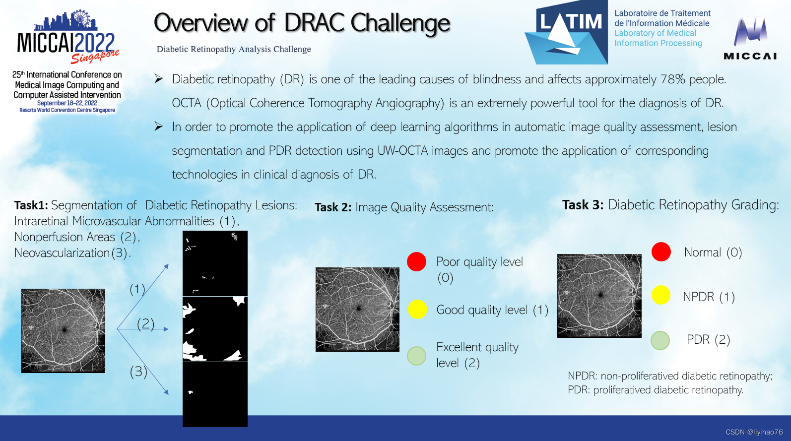
Overview of DRAC Challenge

The ultra-wide OCTA can non-invasively detect the changes of DR neovascularization, thus it is an important imaging modality to help ophthalmologist diagnose PDR. However, there are currently no works capable of automatic DR analysis using UW-OCTA. In the process of DR analysis, the image quality of UW-OCTA needs to be assessed first, and the images with better imaging quality are selected. Then DR analysis is performed, such as lesion segmentation and PDR detection. Thus, it is crucial to build a flexible and robust model to realize automatic image quality assessment, lesion segmentation and PDR detection.

In order to promote the application of machine learning and deep learning algorithms in automatic image quality assessment, lesion segmentation and PDR detection using UW-OCTA images, and promote the application of corresponding technologies in clinical diagnosis of DR, we provide a standardized ultra-wide (swept-source) optical coherence tomography angiography (UW-OCTA) data set for testing the effectiveness of various algorithms. With this dataset, different algorithms can test their performance and make a fair comparison with other algorithms. We believe this dataset is an important milestone in automatic image quality assessment, lesion segmentation and DR grading.

The challenge DRAC22 is a first edition associated with MICCAI 2022. Three tasks are proposed (participants can choose to participate in one or all three tasks):

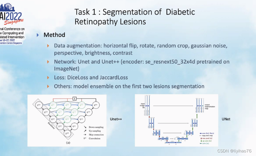
Task 1: Segmentation of Diabetic Retinopathy Lesions.
Task 2: Image Quality Assessment.
Task 3: Diabetic Retinopathy Grading.

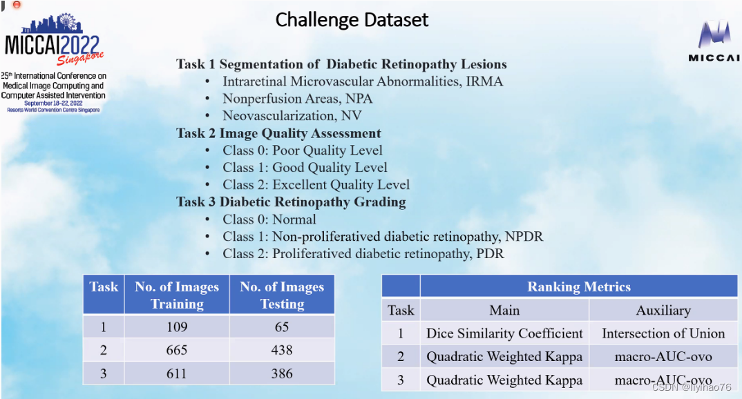
Training and Testing Data

Task 1: Segmentation of Diabetic Retinopathy Lesions: Training set consists of 109 images and corresponding labels.
The dataset contains three different Diabetic Retinopathy Lesions: Intraretinal Microvascular Abnormalities (1), Nonperfusion Areas (2), Neovascularization(3).
Task 2: Image Quality Assessment: Training set consists of 665 images and corresponding labels in CSV file.
The dataset contains three different image quality levels: Poor quality level (0), Good quality level (1), Excellent quality level (2).
Task 3: Diabetic Retinopathy Grading: Training set consists of 611 images and corresponding labels in CSV file.
The dataset contains three different diabetic retinopathy grades: Normal (0), NPDR (1), PDR (2).
NPDR: non-proliferatived diabetic retinopathy; PDR: proliferatived diabetic retinopathy.

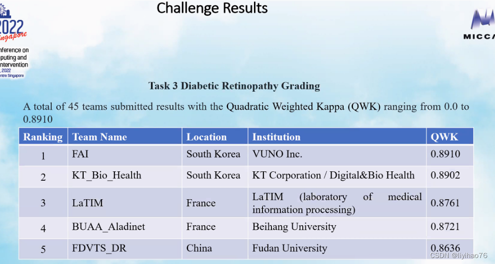
Challenge ranking

在这里插入图片描述

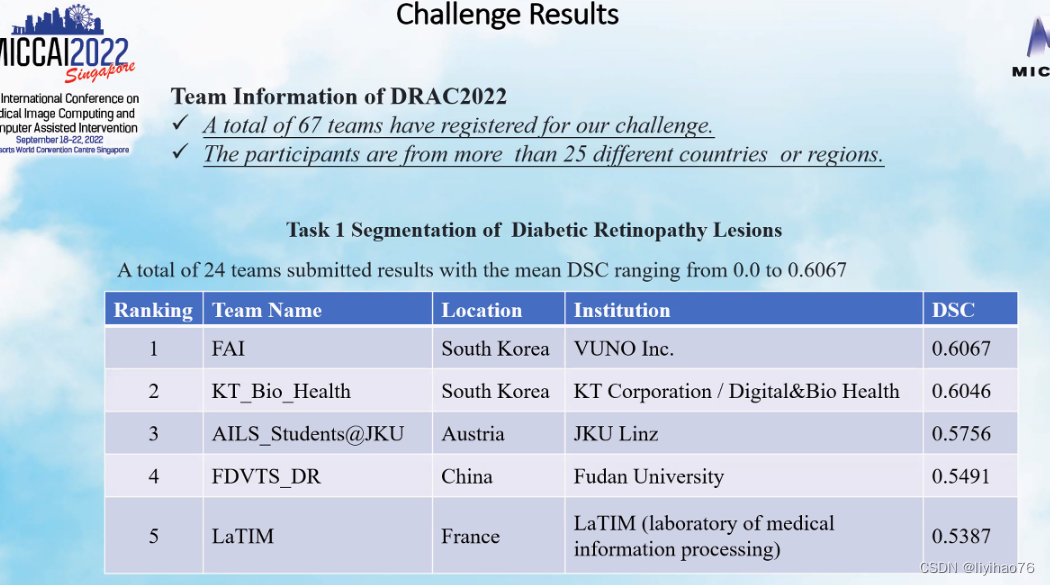
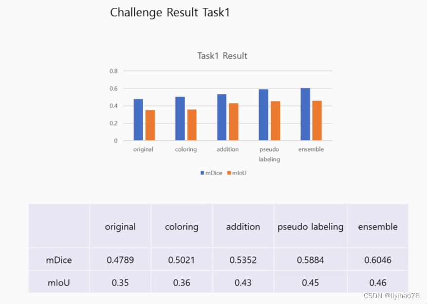
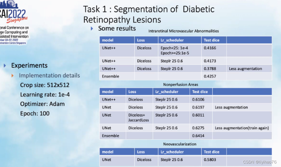
Task 1: Segmentation of Diabetic Retinopathy Lesions

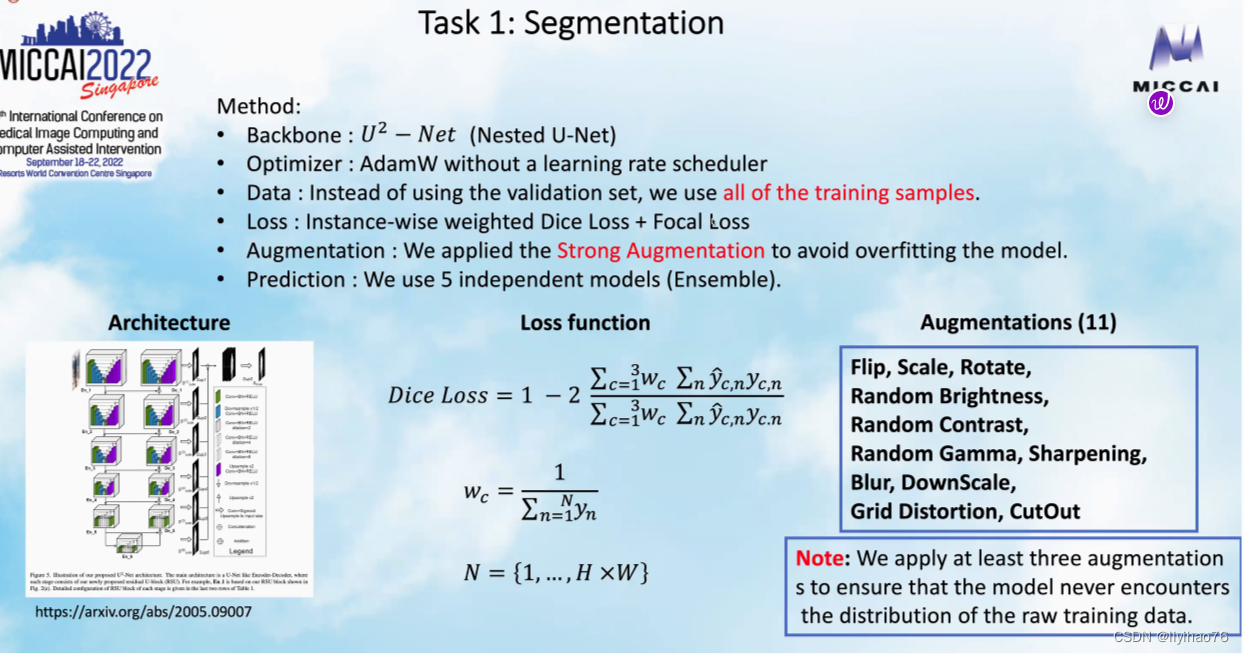
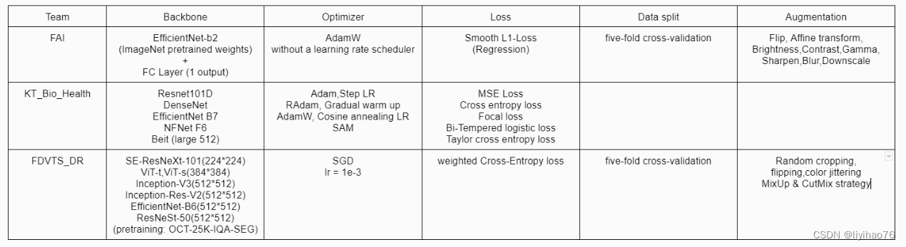
Configuration overview

在这里插入图片描述

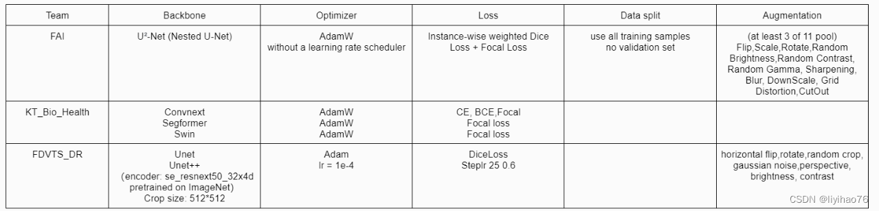
Team: FAI Highlights

使用所有的数据训练，不使用验证集，为此需要强数据增强（Training with all data, without using the validation set, for which strong data augmentation is required）
使用weighted Dice Loss进行多分类分割，而不是3个二分割模型（Multiclassification segmentation using weighted Dice Loss instead of 3 binary segmentation models）
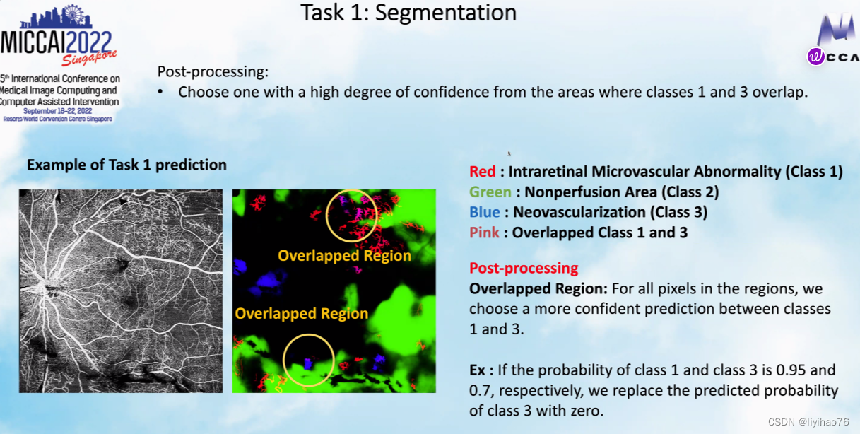
为了解决多分类label之间的重叠，使用了后处理（To resolve the overlap between multiple classification labels, post-processing is used）

Team: KT_BiO_Health Highlights

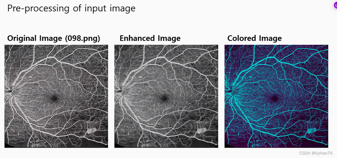
预处理：使用图像增强和彩色化，提高了分割和分类的结果，怎样做的？（Pre-processing：Using image enhancement and colorization improves the results of segmentation and classification, how is it done?）
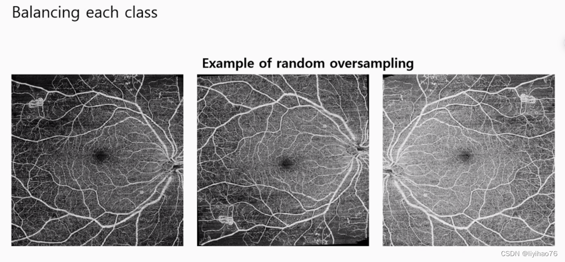
为了解决类不平衡问题，使用了过采样来产生数据（To solve the class imbalance problem, oversampling is used to generate the data）
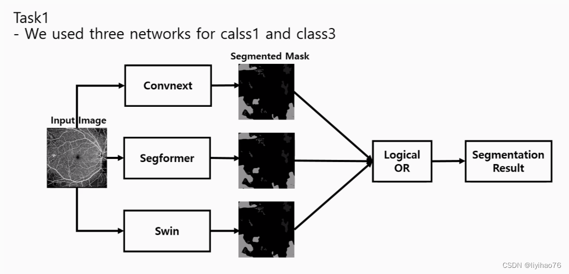
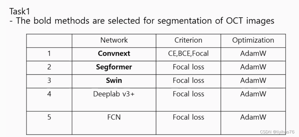
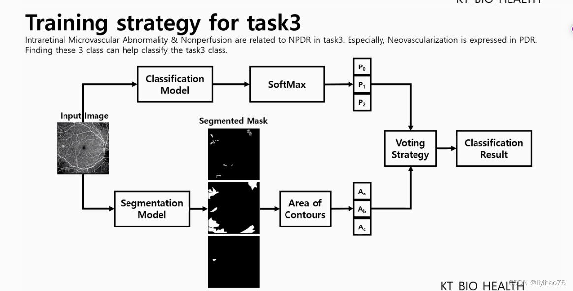
使用三支路网络来融合不同模型的输出结果（Use a three-branch network to fuse the outputs of different models）

Team: FDVTS Highlights

使用了STEPLR学习率衰减策略（STEPLR learning rate decay strategy is used）

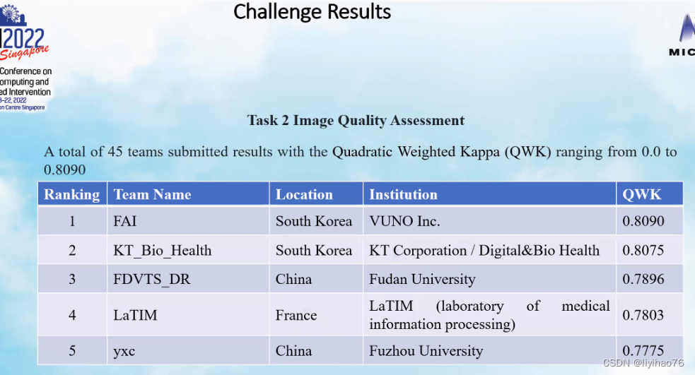
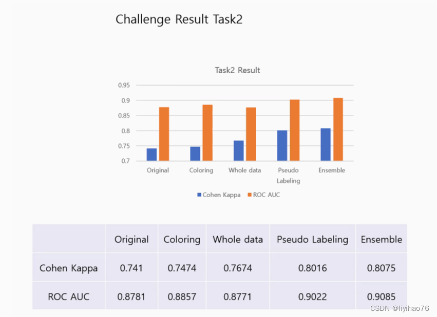
Task 2: Image Quality Assessment

Configuration overview

在这里插入图片描述

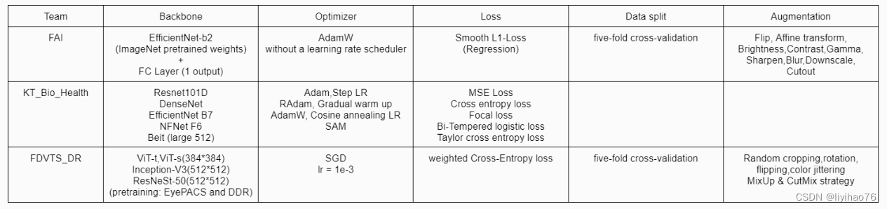
Team: FAI Highlights

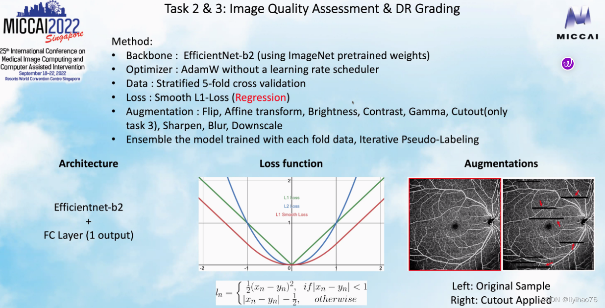
使用回归来完成分类任务，为什么？（Use regression for classification tasks, why?）在分类网络之后加一层变成回归网络，并使用回归损失函数. （Add a layer after the classification network to become a regression network and use the regression loss function.）
五折交叉验证，并对不同折训练出来的模型进行集成（Five-fold cross-validation and ensemble the models trained in different folds）
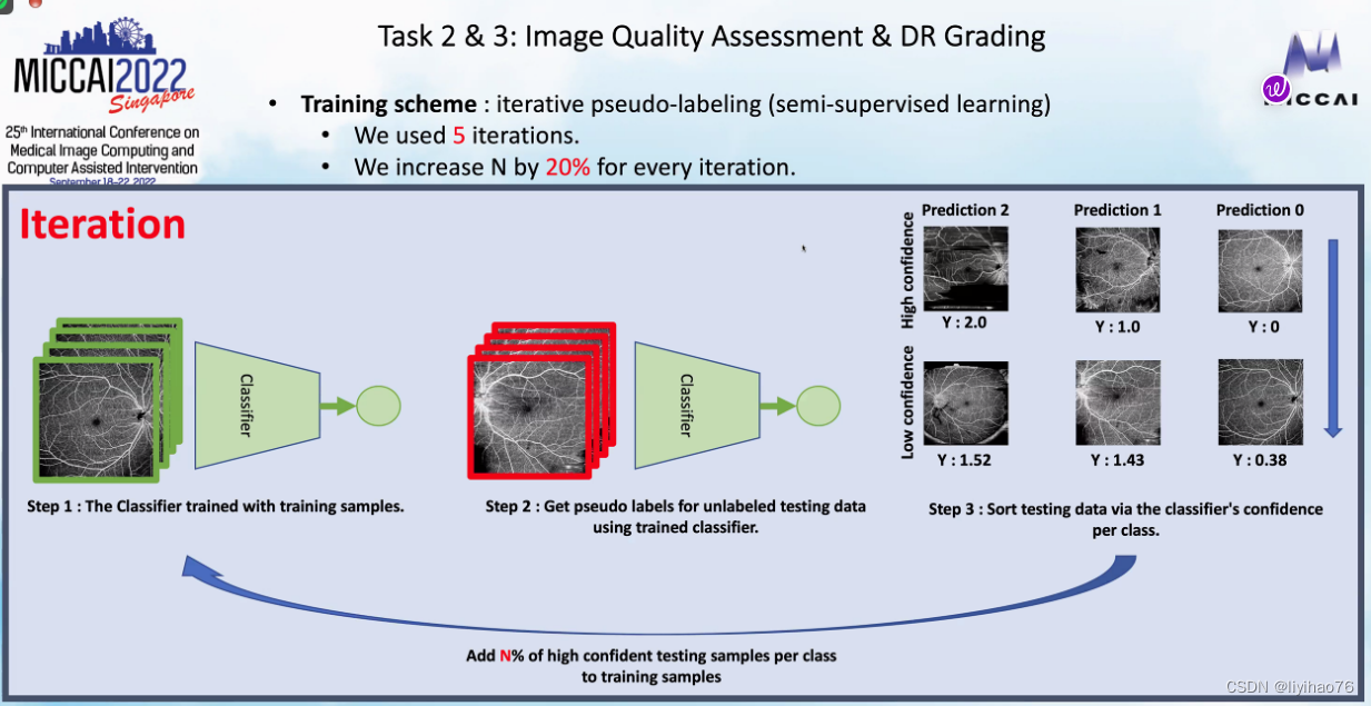
伪标签：迭代，每次选出高置信度的预测结果产生伪标签并且每次产生的伪标签数量都会增加（Pseudolabeling: iteratively, each time a high confidence prediction is selected to generate a pseudolabel and the number of pseudolabels generated is increased each time.）

在这里插入图片描述

Team: KT_BiO_Health Highlights

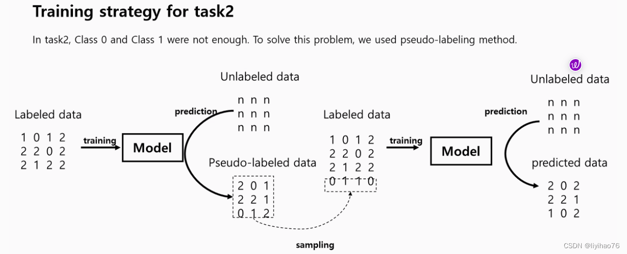
伪标签策略：因为训练集中label0和label1的数量比较少，所以将预测出的0和1数据作为伪标签加入到训练集中（Pseudo-labeling strategy: Because the number of label0 and label1 in the training set is relatively small, the predicted 0 and 1 data are added to the training set as pseudo-labels.）

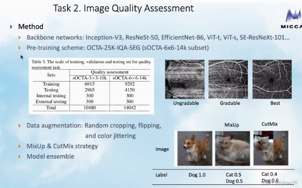
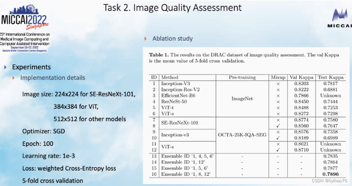
Team: FDVTS Highlights

使用额外的数据集来进行预训练. （Use additional datasets for pre-training）
pre-training dataset from: A Deep Learning-based Quality Assessment and Segmentation System with a Large-scale Benchmark Dataset for Optical Coherence Tomographic Angiography Image
使用了MixUp和CutMix的策略（MixUp and CutMix strategies are used）
cutmix

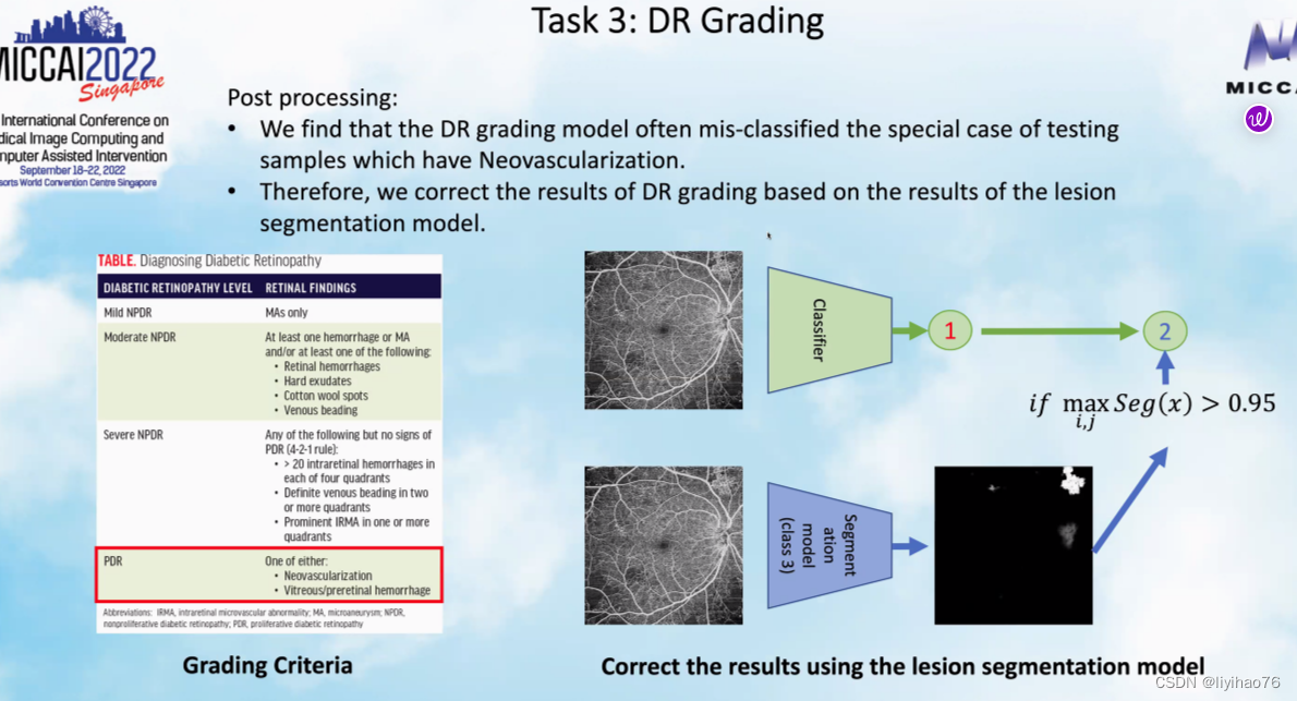
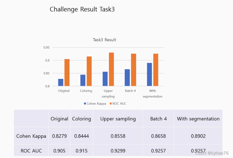
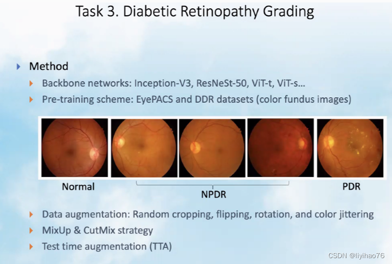
Task 3: Diabetic Retinopathy Grading

Configuration overview

在这里插入图片描述

Team: FAI Highlights

糖尿病性视网膜病变的分类和分割结果之间存在着一些联系，具有某些病理特征的病人大概率是PDR。所以对于分类结果为1的某些数据，如果它的分割概率大于0.95，我们将其的分类结果改为2.（There is some connection between the classification and segmentation results of diabetic retinopathy, and patients with certain pathological features have a high probability of being PDR. so for some data with a classification result of 1, we changed its classification result to 2 if its segmentation probability is greater than 0.95.）

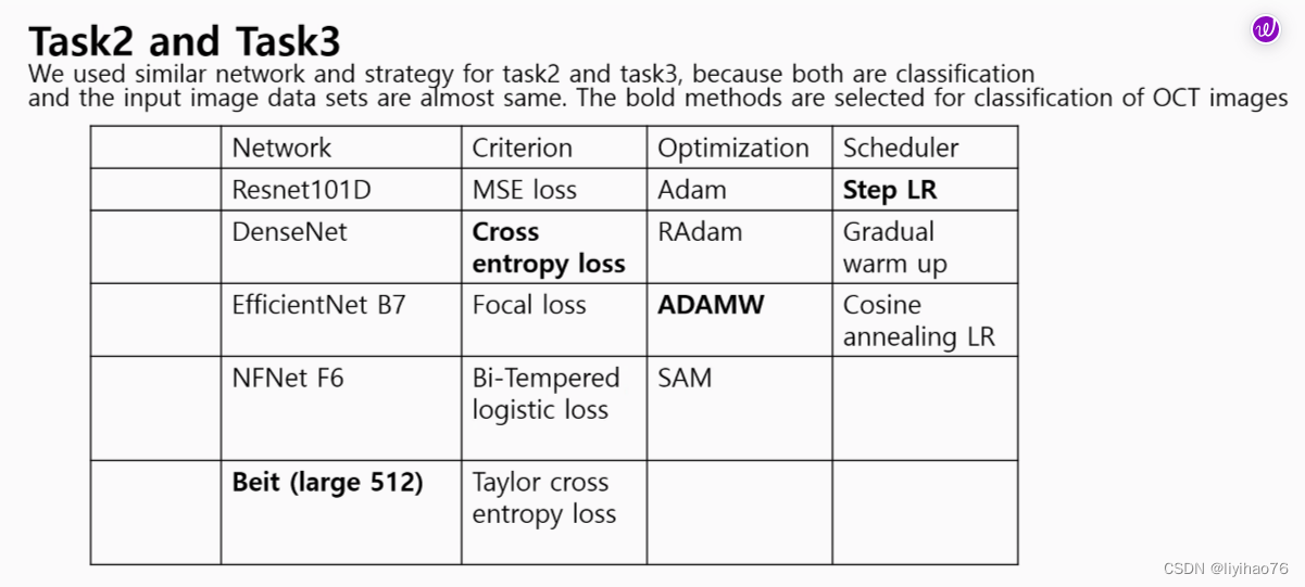
Team: KT_BiO_Health Highlights

分割的结果加入到分类里（The result of the segmentation is added to the classification）

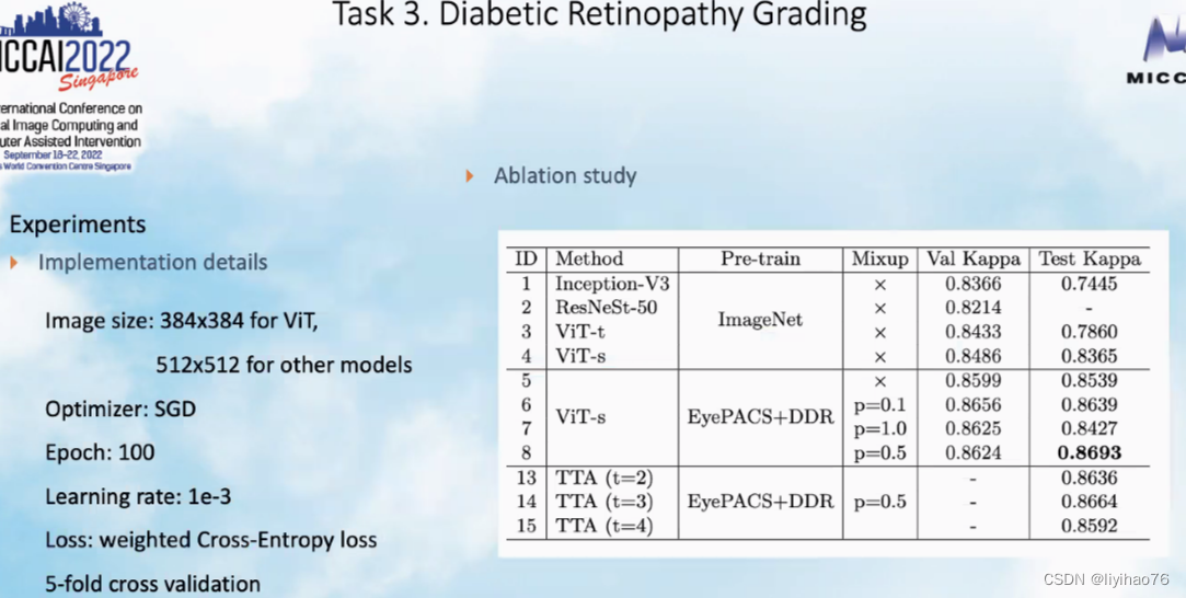
Team: FDVTS Highlights

使用额外的数据集来进行预训练. （Use additional datasets for pre-training）
pre-training dataset from: Diabetic Retinopathy Detection
使用了Test-Time Augmentation策略（Test-Time Augmentation strategy is used）

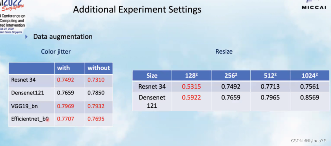
Team: DRIMGA Highlights

网络输入大小的测试，如果较小的size和大size的表现差不多，我们可以减小网络的输入大小来提高batchsize的数量。（The network input size test, if the smaller size and the larger size perform about the same, we can reduce the input size of the network to increase the number of batchsize.）
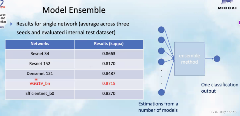
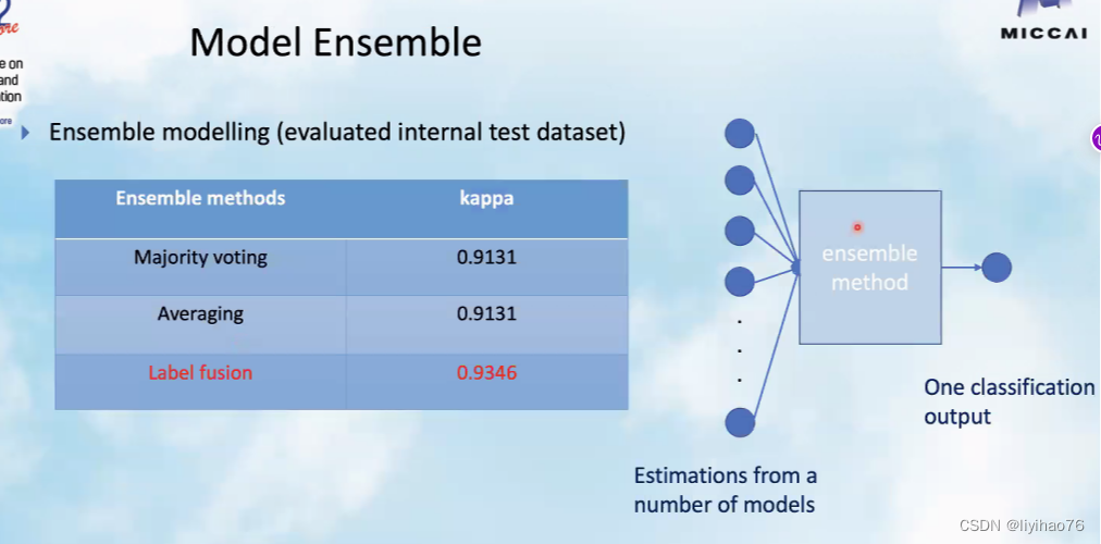
除了投票，平均的模型ensemble方法，我们还可以使用late fusion来让模型自动学习模型权重。（In addition to voting, the average model ensemble method, we can also use late fusion to allow the model to automatically learn model weights.）

在这里插入图片描述

Conclusions

优化器的选择：第一名和第二名的队伍都使用了AdamW优化器，值得测试（Optimizer selection: both the first and second place teams used the AdamW optimizer, which is worth testing）
挑战赛技巧：利用分割的结果提高分类任务的表现. （Challenging trick: Using segmentation results to improve performance on classification tasks.）
对于分类和分割任务，模型集成是获取好成绩的必要步骤。模型集成有很多策略：投票，均值，取或集，权重自动学习…（For classification and segmentation tasks, model ensemble is a necessary step to get good results. There are many strategies for model ensemble: voting, mean, take or set, weight automatic learning…）
伪标签可以显著提高分类任务的表现，伪标签的产生可以有不同的策略。（Pseudolabeling can significantly improve the performance of classification tasks, and pseudolabeling can be generated with different strategies.）

Annexe

U2-Net

github
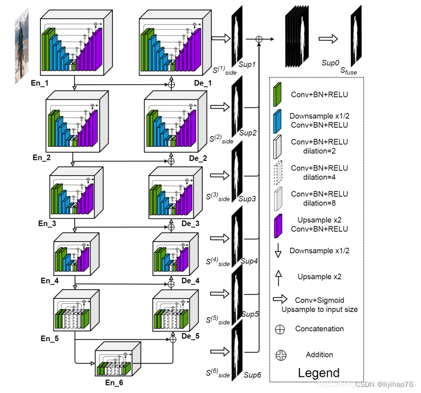
U2net是基于unet提出的一种新的网络结构，同样基于encode-decode，作者参考FPN，Unet，在此基础之上提出了一种新模块RSU(ReSidual U-blocks) 经过测试，对于分割物体前背景取得了惊人的效果。同样具有较好的实时性，经过测试在P100上前向时间仅为18ms(56fps)。
下面是对U2net的一个介绍：

首先还是贴一下网络结构：
在这里插入图片描述
U2Net论文解读及代码测试
 图像分割之U2-Net介绍
其实这个网络结构以及把一整个u2net完整的表示出来了，作者提出了一种名为RSU的新模块。对于每个RSU本身就是一个小号的Unet，最后所有的RSU用一种类似FPN的结构连接在一起。类似down-top top-down。通过这种方式来增加多尺度能力。获得了极为优秀的分割结果。

下面是RSU结构：
在这里插入图片描述
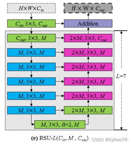
从这个结构可以很容易的看出，所谓的RSU其实就是一个很简单的Unet

作者通过类似FPN的结构，将多个Unet输出结果进行组合。最后进行合并，得到mask，通过多个loss在不同层的表现来进行更新。取得了非常理想的效果

下面是整个U2net代码细节的介绍：

class U2NET(nn.Module):

    def __init__(self,in_ch=3,out_ch=1):
        super(U2NET,self).__init__()
        self.stage1 = RSU7(in_ch,32,64)
		#对于每一个RSU来说，本质其实就是一个Unet，多个下采样多个上采样

        self.pool12 = nn.MaxPool2d(2,stride=2,ceil_mode=True)
        self.stage2 = RSU6(64,32,128)
        self.pool23 = nn.MaxPool2d(2,stride=2,ceil_mode=True)
        self.stage3 = RSU5(128,64,256)
        self.pool34 = nn.MaxPool2d(2,stride=2,ceil_mode=True)
        self.stage4 = RSU4(256,128,512)
        self.pool45 = nn.MaxPool2d(2,stride=2,ceil_mode=True)
        self.stage5 = RSU4F(512,256,512)
        self.pool56 = nn.MaxPool2d(2,stride=2,ceil_mode=True)
        self.stage6 = RSU4F(512,256,512)
        # decoder
        self.stage5d = RSU4F(1024,256,512)
        self.stage4d = RSU4(1024,128,256)
        self.stage3d = RSU5(512,64,128)
        self.stage2d = RSU6(256,32,64)
        self.stage1d = RSU7(128,16,64)
        self.side1 = nn.Conv2d(64,out_ch,3,padding=1)
        self.side2 = nn.Conv2d(64,out_ch,3,padding=1)
        self.side3 = nn.Conv2d(128,out_ch,3,padding=1)
        self.side4 = nn.Conv2d(256,out_ch,3,padding=1)
        self.side5 = nn.Conv2d(512,out_ch,3,padding=1)
        self.side6 = nn.Conv2d(512,out_ch,3,padding=1)
        self.outconv = nn.Conv2d(6,out_ch,1)

    def forward(self,x):

        hx = x
        #stage 1
        hx1 = self.stage1(hx)
        #通过一个个Unet得到相应的mask
        hx = self.pool12(hx1)
        #stage 2
        hx2 = self.stage2(hx)
        hx = self.pool23(hx2)
        #stage 3
        hx3 = self.stage3(hx)
        hx = self.pool34(hx3)
        #stage 4
        hx4 = self.stage4(hx)
        hx = self.pool45(hx4)
        #stage 5
        hx5 = self.stage5(hx)
        hx = self.pool56(hx5)
        #stage 6
        hx6 = self.stage6(hx)
        hx6up = _upsample_like(hx6,hx5)
        #-------------------- decoder --------------------
        hx5d = self.stage5d(torch.cat((hx6up,hx5),1))
        #这里类似FPN。每个block的输出结果和上一个（下一个block）结果做融合（cat），然后输出。
        hx5dup = _upsample_like(hx5d,hx4)
        #由于每个block做了下采样，为了resize到原图，需要做一个上采样，这里作者直接用的双线性插值做的上采样
        hx4d = self.stage4d(torch.cat((hx5dup,hx4),1))
        hx4dup = _upsample_like(hx4d,hx3)
        hx3d = self.stage3d(torch.cat((hx4dup,hx3),1))
        hx3dup = _upsample_like(hx3d,hx2)
        hx2d = self.stage2d(torch.cat((hx3dup,hx2),1))
        hx2dup = _upsample_like(hx2d,hx1)
        hx1d = self.stage1d(torch.cat((hx2dup,hx1),1))


        #side output
        d1 = self.side1(hx1d)
		#这里本质就是把每一个block输出结果，转换成WxHx1的mask最后过一个sigmod就可以得到每个block输出的概率图。
        d2 = self.side2(hx2d)
        d2 = _upsample_like(d2,d1)

        d3 = self.side3(hx3d)
        d3 = _upsample_like(d3,d1)

        d4 = self.side4(hx4d)
        d4 = _upsample_like(d4,d1)

        d5 = self.side5(hx5d)
        d5 = _upsample_like(d5,d1)

        d6 = self.side6(hx6)
        d6 = _upsample_like(d6,d1)

        d0 = self.outconv(torch.cat((d1,d2,d3,d4,d5,d6),1))
		#6个blovk cat一起之后做特征融合，然后再做输出，结果就是d0的结果，其他的输出都是为了计算loss
        return F.sigmoid(d0), F.sigmoid(d1), F.sigmoid(d2), F.sigmoid(d3), F.sigmoid(d4), F.sigmoid(d5), F.sigmoid(d6)

具体的对于每个RSU来说：

class RSU7(nn.Module):#UNet07DRES(nn.Module):

    def __init__(self, in_ch=3, mid_ch=12, out_ch=3):
        super(RSU7,self).__init__()

        self.rebnconvin = REBNCONV(in_ch,out_ch,dirate=1)

        self.rebnconv1 = REBNCONV(out_ch,mid_ch,dirate=1)
        self.pool1 = nn.MaxPool2d(2,stride=2,ceil_mode=True)

        self.rebnconv2 = REBNCONV(mid_ch,mid_ch,dirate=1)
        self.pool2 = nn.MaxPool2d(2,stride=2,ceil_mode=True)

        self.rebnconv3 = REBNCONV(mid_ch,mid_ch,dirate=1)
        self.pool3 = nn.MaxPool2d(2,stride=2,ceil_mode=True)

        self.rebnconv4 = REBNCONV(mid_ch,mid_ch,dirate=1)
        self.pool4 = nn.MaxPool2d(2,stride=2,ceil_mode=True)

        self.rebnconv5 = REBNCONV(mid_ch,mid_ch,dirate=1)
        self.pool5 = nn.MaxPool2d(2,stride=2,ceil_mode=True)

        self.rebnconv6 = REBNCONV(mid_ch,mid_ch,dirate=1)

        self.rebnconv7 = REBNCONV(mid_ch,mid_ch,dirate=2)

        self.rebnconv6d = REBNCONV(mid_ch*2,mid_ch,dirate=1)
        self.rebnconv5d = REBNCONV(mid_ch*2,mid_ch,dirate=1)
        self.rebnconv4d = REBNCONV(mid_ch*2,mid_ch,dirate=1)
        self.rebnconv3d = REBNCONV(mid_ch*2,mid_ch,dirate=1)
        self.rebnconv2d = REBNCONV(mid_ch*2,mid_ch,dirate=1)
        self.rebnconv1d = REBNCONV(mid_ch*2,out_ch,dirate=1)

    def forward(self,x):

        hx = x
        hxin = self.rebnconvin(hx)

        hx1 = self.rebnconv1(hxin)
        hx = self.pool1(hx1)

        hx2 = self.rebnconv2(hx)
        hx = self.pool2(hx2)

        hx3 = self.rebnconv3(hx)
        hx = self.pool3(hx3)

        hx4 = self.rebnconv4(hx)
        hx = self.pool4(hx4)

        hx5 = self.rebnconv5(hx)
        hx = self.pool5(hx5)

        hx6 = self.rebnconv6(hx)

        hx7 = self.rebnconv7(hx6)

        hx6d =  self.rebnconv6d(torch.cat((hx7,hx6),1))
        hx6dup = _upsample_like(hx6d,hx5)
		#双线性差值做的上采样
        hx5d =  self.rebnconv5d(torch.cat((hx6dup,hx5),1))
        hx5dup = _upsample_like(hx5d,hx4)

        hx4d = self.rebnconv4d(torch.cat((hx5dup,hx4),1))
        hx4dup = _upsample_like(hx4d,hx3)

        hx3d = self.rebnconv3d(torch.cat((hx4dup,hx3),1))
        hx3dup = _upsample_like(hx3d,hx2)

        hx2d = self.rebnconv2d(torch.cat((hx3dup,hx2),1))
        hx2dup = _upsample_like(hx2d,hx1)

        hx1d = self.rebnconv1d(torch.cat((hx2dup,hx1),1))

        return hx1d + hxin

对应结构图本质其实是这样的：
在这里插入图片描述
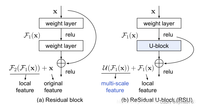
RSU和ResNet的残差结构其实非常的相似。只不过将权重层换成了Unet而已。

最后我们来看下loss：

由于作者把U2net分成了多个block，每个block输出一个loss，那么最后整个模型的loss自然就是这样的
在这里插入图片描述
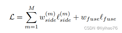
然后带了一堆的解释，本质其实就是7个loss相加（6个block输出结果加1个特征融合后的结果）：

def muti_bce_loss_fusion(d0, d1, d2, d3, d4, d5, d6, labels_v):

	loss0 = bce_loss(d0,labels_v)
	loss1 = bce_loss(d1,labels_v)
	loss2 = bce_loss(d2,labels_v)
	loss3 = bce_loss(d3,labels_v)
	loss4 = bce_loss(d4,labels_v)
	loss5 = bce_loss(d5,labels_v)
	loss6 = bce_loss(d6,labels_v)

	loss = loss0 + loss1 + loss2 + loss3 + loss4 + loss5 + loss6
	print("l0: %3f, l1: %3f, l2: %3f, l3: %3f, l4: %3f, l5: %3f, l6: %3f\n"%(loss0.data[0],loss1.data[0],loss2.data[0],loss3.data[0],loss4.data[0],loss5.data[0],loss6.data[0]))

	return loss0, loss

#每个mask计算二值交叉熵最后相加
d0, d1, d2, d3, d4, d5, d6 = net(inputs_v)
loss2, loss = muti_bce_loss_fusion(d0, d1, d2, d3, d4, d5, d6, labels_v)

loss.backward()
optimizer.step()

AdamW

Adamw 即 Adam + weight decate ,效果与 Adam + L2正则化相同,但是计算效率更高,因为L2正则化需要在loss中加入正则项,之后再算梯度,最后在反向传播,而Adamw直接将正则项的梯度加入反向传播的公式中,省去了手动在loss中加正则项这一步

torch.optim.AdamW(params, lr=0.001, betas=(0.9, 0.999), eps=1e-08, weight_decay=0.01, amsgrad=False, *, maximize=False, foreach=None, capturable=False)

目标检测回归损失函数——L1、L2、smooth L1

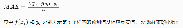
L1 Loss
L1 Loss也称为平均绝对值误差（MAE），是指模型预测值f(x)和真实值y之间绝对差值的平均值，公式如下：

在这里插入图片描述
曲线分布如下：

在这里插入图片描述
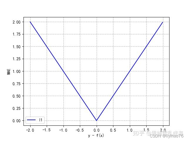
MAE函数虽然连续，但是在0处不可导。而且MAE的导数为常数，所以在较小的损失值时，得到的梯度也相对较大，可能造成模型震荡不利于收敛。

L2 Loss
L2 Loss也称为均方误差（MSE），是指模型预测值f(x)和真实值y之间差值平方的平均值，公式如下：

曲线分布如下：

在这里插入图片描述

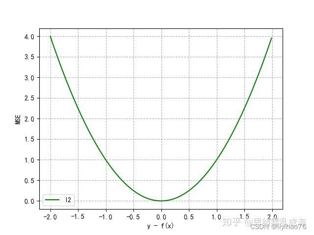
由于采用平方运算，当预测值和真实值的差值大于1时，会放大误差。尤其当函数的输入值距离中心值较远的时候，使用梯度下降法求解的时候梯度很大，可能造成梯度爆炸。同时当有多个离群点时，这些点可能占据Loss的主要部分，需要牺牲很多有效的样本去补偿它，所以MSE损失函数受离群点的影响较大。

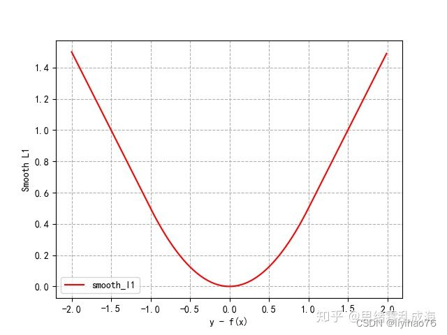
Smooth L1 Loss
简单的说Smooth L1就是一个平滑版的L1 Loss，其公式如下：

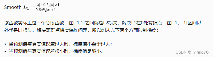
曲线分布如下：

StepLR

torch.optim.lr_scheduler.StepLR(optimizer, step_size, gamma=0.1, last_epoch=- 1, verbose=False)

optimizer （Optimizer）：要更改学习率的优化器；
step_size（int）：每训练step_size个epoch，更新一次参数；
gamma（float）：更新lr的乘法因子；
last_epoch （int）：最后一个epoch的index，如果是训练了很多个epoch后中断了，继续训练，这个值就等于加载的模型的epoch。默认为-1表示从头开始训练，即从epoch=1开始。

Example

>>> # Assuming optimizer uses lr = 0.05 for all groups
>>> # lr = 0.05     if epoch < 30
>>> # lr = 0.005    if 30 <= epoch < 60
>>> # lr = 0.0005   if 60 <= epoch < 90
>>> # ...
>>> scheduler = StepLR(optimizer, step_size=30, gamma=0.1)
>>> for epoch in range(100):
>>>     train(...)
>>>     validate(...)
>>>     scheduler.step()

Test-Time Augmentation

数据增强是一种用于提高计算机视觉问题神经网络模型的性能和减少泛化误差的技术。当使用拟合模型进行预测时，也可以应用图像数据增强技术，以允许模型对测试数据集中每幅图像的多个不同版本进行预测。对增强图像的预测可以取平均值，从而获得更好的预测性能。

定义:TTA(Test Time Augmentation):测试时数据增强
方法:测试时将原始数据做不同形式的增强,然后取结果的平均值作为最终结果
作用:可以进一步提升最终结果的精度。
在这里插入图片描述
Image Test Time Augmentation with PyTorch!

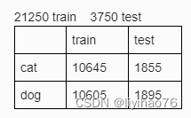
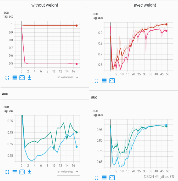
Weighted loss

原数据集 25000 images = 12500 cats + 12500 dogs
X_train,X_test,y_train,y_test = train_test_split(train_path_list,label_list,test_size = 0.15,random_state = 1)
在这里插入图片描述
取dog训练集图片的百分之一

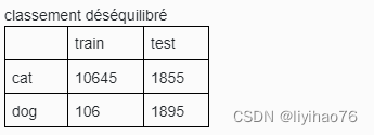
criterion = torch.nn.BCEWithLogitsLoss(pos_weight=torch.tensor([100.0])).cuda()

在这里插入图片描述

liyihao76

关注

1
点赞
踩
3

收藏

觉得还不错? 一键收藏
4
评论
DRAC2022比赛总结+前五解决方案

DRAC2022 比赛总结
复制链接

扫一扫

专栏目录

DRAC2022比赛总结+前五解决方案

Contents

Introduction

Overview of DRAC Challenge

Challenge ranking

Task 1: Segmentation of Diabetic Retinopathy Lesions

Configuration overview

Team: FAI Highlights

Team: KT_BiO_Health Highlights

Team: FDVTS Highlights

Task 2: Image Quality Assessment

Configuration overview

Team: FAI Highlights

Team: KT_BiO_Health Highlights

Team: FDVTS Highlights

Task 3: Diabetic Retinopathy Grading

Configuration overview

Team: FAI Highlights

Team: KT_BiO_Health Highlights

Team: FDVTS Highlights

Team: DRIMGA Highlights

Conclusions

Annexe

U2-Net

AdamW

目标检测回归损失函数——L1、L2、smooth L1

StepLR

Test-Time Augmentation

Weighted loss

“相关推荐”对你有帮助么？