从Jaccard到BERT：语义检索的度量手段

原文标题：Semantic Search: Measuring Meaning From Jaccard to Bert
作者：James Briggs
原文地址：https://towardsdatascience.com/semantic-search-measuring-meaning-from-jaccard-to-bert-a5aca61fc325

注：只挑选了干货部分进行翻译

前言

相似性搜索（Similarity search）是人工智能和机器学习中发展最快的领域之一。其核心是将相关信息片段匹配在一起的过程。

相似性搜索是一个复杂的主题，有无数的技术来构建有效的搜索引擎。在本文中，我们将介绍这些技术中最有趣、最强大的，特别关注语义检索（semantic search）。我们将学习它们如何工作，它们的优势，以及如何自己实现它们。

---

1. 传统搜索

• Jaccard Similarity
• w-shingling
• Pearson Similarity
• Levenshtein距离
• 标准化谷歌距离（Normalized Google Distance）

所有这些都是用于相似性搜索的优秀指标，其中我们将介绍三个最流行的指标：Jaccard相似性、w-shingling和Levenshtein距离。

1.1 Jaccard Similarity

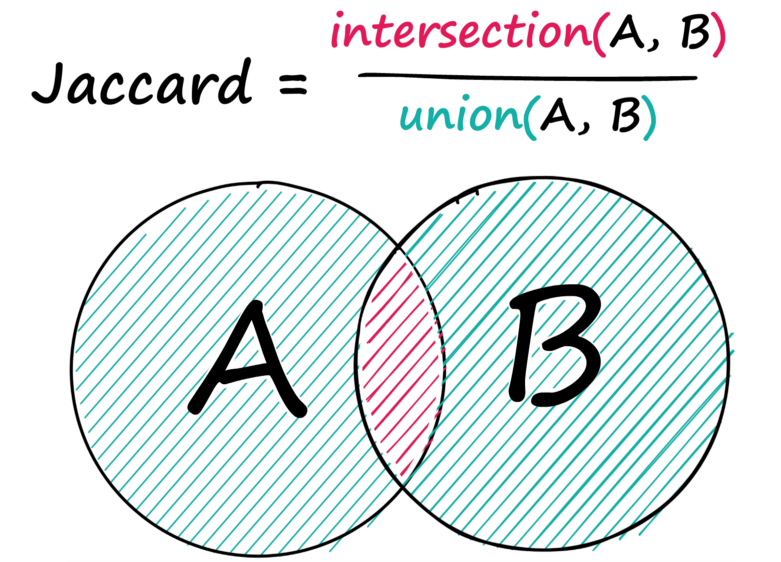
Jaccard相似性是一个简单，但有些时候很有用的相似性度量手段。
给定两个序列，A和B，我们求出两者之间共有的元素的数量，然后除以两个序列中的元素总数。

Jaccard相似度度量两个序列在两个序列的并集上的交集：

下面是一段示例代码：

a = [0, 1, 2, 3, 3, 3, 4]
b = [7, 6, 5, 4, 4, 3]

# convert to sets
a = set(a)
b = set(b)

# find the number of shared values between sets
shared = a.intersection(b)

# find the total number of values in both sets
total = a.union(b)

# and calculate Jaccard similarity
len(shared) / len(total)

在这里，我们确定了两个序列之间的两个共享唯一整数，3和4，这两个序列中总共有10个整数，其中8个是唯一值
由$2/8$ 得到Jaccard相似性得分为0.25。

我们也可以对文本数据执行相同的操作，我们所做的就是用单词替换整数。
计算两个句子a和b之间的Jaccard相似度：

a = "his thought process was on so many levels that he gave himself a phobia of heights".split()
b = "there is an art to getting your way and throwing bananas on to the street is not it".split()
c = "it is not often you find soggy bananas on the street".split()

a = set(a)
b = set(b)
c = set(c)

def jac(x: set, y: set):
    shared = x.intersection(y)  # selects shared tokens only
    return len(shared) / len(x.union(y))  # union adds both sets together

jac(a, b) # 0.03225806451612903
jac(b, c) # 0.35

我们发现句子b和c的得分要高得多，正如我们预期的那样。现在，它并不是完美的——两个除了“the”、“a”、“is”等词之外什么都没有的句子可能会返回很高的Jaccard分数，尽管语义不同。

这些缺点可以通过预处理技术部分解决，如使用停用词表，词干/词形还原等。然而，我们很快就会看到，有些方法完全避免了这些问题。

1.2 w-Shingling

另一种类似的技术是w-Shingling。
w-Shingling使用完全相同的取交集，并集逻辑，但使用“shingles”。
个人理解就是n-grams

The w denotes the number of tokens in each shingle in the set.

句子A的2-shingle看起来像：a = {‘his thought’, ‘thought process’, ‘process is’, …}
就是取了句子的2-gram。

# 句子分词
a = "his thought process was on so many levels that he gave himself a phobia of heights".split()
b = "there is an art to getting your way and throwing bananas on to the street is not it".split()
c = "it is not often you find soggy bananas on the street".split()

a_shingle = set([' '.join([a[i], a[i+1]]) for i in range(len(a)) if i != len(a)-1])
b_shingle = set([' '.join([b[i], b[i+1]]) for i in range(len(b)) if i != len(b)-1])
c_shingle = set([' '.join([c[i], c[i+1]]) for i in range(len(c)) if i != len(c)-1])

# 仍然可用杰卡德距离的公式计算，只不过每个元素由单词变为了2-gram
jac(a_shingle, b_shingle)  # 0.0

jac(b_shingle, c_shingle)  # 0.125

# 展示两句中匹配的shingles
b_shingle.intersection(c_shingle)  
# {'bananas on', 'is not', 'the street'}

1.3 Levenshtein Distance

莱文斯坦距离，又称Levenshtein距离，是编辑距离的一种。指两个字串之间，由一个转成另一个所需的最少编辑操作次数。允许的编辑操作包括将一个字符替换成另一个字符，插入一个字符，删除一个字符。

这是一道经典的动态规划算法题，可前往力扣自行练习。
题目链接：https://leetcode-cn.com/problems/edit-distance/。

Levenshtein距离公式：

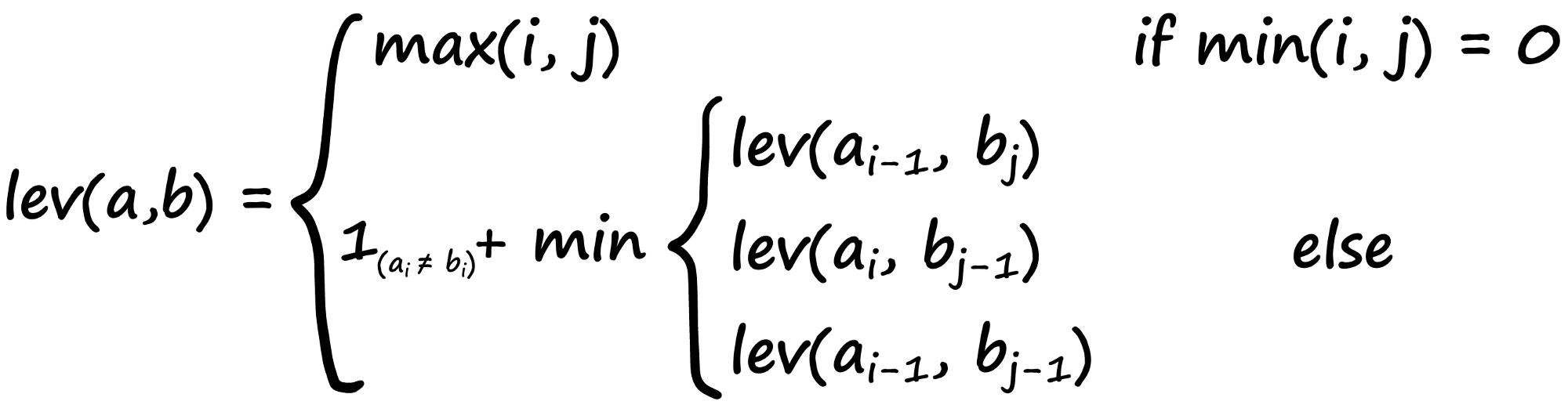
变量a和b代表两个字符串，i和j分别代表a和b中的字符位置。

下标从1开始，索引0将代表空字符串

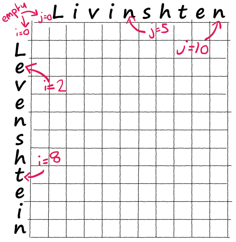
使用Wagner-Fischer matrix来计算两个字符串的莱温斯坦距离。

a = ' Levenshtein'
b = ' Livinshten'  # we include empty space at start of each word
import numpy as np
# initialize empty zero array
lev = np.zeros((len(a), len(b)))

lev[i][j] 表示a[0:i]变换到b[0:j]的最小操作次数。

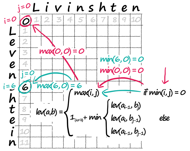
首先处理dp表的边界。很容易理解，一个空的字符串要变成另一个字符串，操作数必然是非空字符串的长度。

for i in range(len(a)):
    for j in range(len(b)):
        # if i or j are 0
        if min([i, j]) == 0:
            # we assign matrix value at position i, j = max(i, j)
            lev[i, j] = max([i, j])

内部元素的计算：

for i in range(len(a)):
    for j in range(len(b)):
        # we did this before (for when i or j are 0)
        if min([i, j]) == 0:
            lev[i, j] = max([i, j])
        else:
            # calculate our three possible operations
            x = lev[i-1, j]    # 删除 
            y = lev[i, j-1]    # 插入
            z = lev[i-1, j-1]  # 替换
            # take the minimum (eg best path/operation)
            lev[i, j] = min([x, y, z])
            # and if our two current characters don't match, add 1
            if a[i] != b[j]:
                # if we have a match, don't add 1
                lev[i, j] += 1

这篇博客没有讲清楚算法的原理，只是用画图展示了计算过程。提供的代码，耗时和内存也很糟糕。

下面讲一讲基本的动态规划思路：
指针$i$指向word1, 指针$j$指向word2

• $dp[0][0]$表示word1和word2都是空的字符串
• $dp[i][j]$表示word1的前i个字符转换成word2的前j个字符所需要的最少操作步数

注意只看操作的word1的字符范围，不看操作后的word1的长度！并且我们始终操作word1。

确定递推公式
当word1[i-1] == word2[j-1]时，什么也不做，dp[i][j] = dp[i-1][j-1]
当word1[i-1] != word2[j-1]时， 有三种情况：
1. 什么时候插入？
已经将word1的前i个字符转换为word2的前j-1个字符了（最小操作数为dp[i][j-1]）
只需在word1的第i个字符后面插入word2[j]
2. 什么时候删除？
已经将word1前i-1个字符转换为word2的前j个字符（最小操作数为dp[i-1][j]）
只需要删除word1[i-1], 相当于dp[i-1][j]加上一次删除操作
3. 什么时候替换?
已经将word1的前i-1个字符转换成word2的前j-1个字符（最小操作数为dp[i-1][j-1]）
只需要将word1的第i个字符替换成word2的第j个字符

2. 向量相似度检索

• TF-IDF
• BM25
• word2vec/doc2vec
• BERT
• USE

这些基于向量的方法是相似度搜索领域的最优方法。
我们将介绍基于TF-IDF、BM25和BERT的方法，因为它们是最常见的方法，并且涵盖稀疏和密集向量表示。

2.1 TF-IDF

信息检索领域的经典方法，诞生于1970s。
关于TF-IDF这部分，也可以参考我的博客：
IR&IE笔记：倒排索引表与布尔模型
IR&IE笔记：向量空间模型与扩展的向量空间模型

TF(term frequency)部分计算一个词语在一个文档中出现的次数，并将其除以该文档中的词语总数。
$TF=\frac{f(q,D)}{f(t,D)}$

• $f(q,D)$: q在文档D中出现的次数
• $f(t,D)$: 文档d的词数

“bananas"是一个比较有信息含量的查询词，计算所有文档的TF('bananas', D)，可以找出"bananas"出现频率较高的文档。但是如果query中还包含了一些常用词呢？如"the”、“is"或"it"这样的词。假如我们搜索"is bananas”，可能含有更多"is"的文档"is is is is is"就会排在更前面。但显然不是我们想要的。

某个单词出现次数越小，那文档中出现此单词的概率越小，则信息量越高。理想情况下，我们希望稀有词，即带有更多信息的词的匹配得分更高。因此我们需要第二个指标IDF，逆向文档频率。

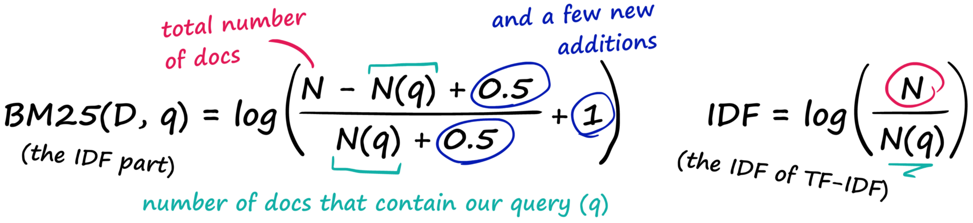
IDF(The Inverse Document Frequency)衡量了一个单词在所有文档中的非常见程度。
$IDF=log\frac{N}{N(q)}$
$N(q)$: 包含词项$q$的文档的数量

如下图所示，假如我们同时搜索"is"和"forest"这两个词，首先计算一次两个词的IDF值，再计算每个文档的TF('is', D)and TF('forest', D)，将TF与IDF相乘得到每篇文档的TF-IDF值。

可以发现，尽管"is"在每篇文档的TF值较大，但IDF值为0，TF-IDF值还是帮助我们找到了信息量更大的，包含"forest"的文档。

原博客提供的代码有误，修正后的代码如下：

a = "purple is the best city in the forest".split()
b = "there is an art to getting your way and throwing bananas on to the street is not it".split()
c = "it is not often you find soggy bananas on the street".split()

import numpy as np

def tfidf(word):
    tf = []
    count_n = 0
    for sentence in [a, b, c]:
        t_count = 0
        # calculate TF
        for x in sentence:
            if word == x:
                t_count += 1
        tf.append(t_count/len(sentence))
        # count number of docs for IDF
        count_n += 1 if word in sentence else 0
    idf = np.log10(len([a, b, c]) / count_n)
    return [round(_tf*idf, 2) for _tf in tf]

tfidf_a, tfidf_b, tfidf_c = tfidf('forest')
print(f"TF-IDF a: {tfidf_a}\nTF-IDF b: {tfidf_b}\nTF-IDF c: {tfidf_c}")

看起来TF-IDF本身就是一个检索算法了，那么，向量相似性检索从哪里来的呢？
根据所有的文档，维护一个词汇表。
一个文档，就可以用其所有单词的TF-IDF值表示成为一个向量，向量的长度为词表大小。

示例代码如下：

vocab = set(a+b+c)
# initialize vectors
vec_a = []
vec_b = []
vec_c = []

for word in vocab:
    tfidf_a, tfidf_b, tfidf_c = tfidf(word)
    vec_a.append(tfidf_a)
    vec_b.append(tfidf_b)
    vec_c.append(tfidf_c)
print(vec_a)
# [0.0, 0.0, 0.0, 0.0, 0.0, 0.48, 0.0, 0.0, 0.48, 0.0, 0.48, 0.48, 0.0, 0.0, 0.0, 0.0, 0.48, 0.0, 0.0, 0.0, 0.0, 0.0, 0.0, 0.0, 0.0]

值得注意的是，vocab的大小很容易在20K+范围内，因此使用这种方法生成的向量非常稀疏，这意味着我们无法编码任何语义。

2.2 BM25

Okapi BM25是TF-IDF的改进算法，基于文档长度对结果进行标准化。
假设我们有两篇500词的文章，发现A提到“丘吉尔”六次，B提到“丘吉尔”十二次——我们是否应该认为A有一半B的相关性？
大概不会。
BM25通过改进TF-IDF的公式解决了这个问题。

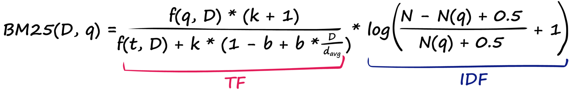
先来看TF部分

再来看IDF部分

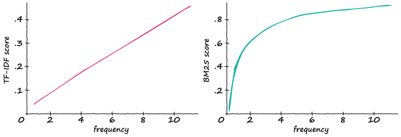
随着查询词在句子中的频率提升，两个算法分数的直观对比如下所示。
TF-IDF分数随着相关单词的数量线性增加。因此，如果频率加倍，TF-IDF分数也会加倍。
而BM25的分数，不会在词频较高时线性增加。

计算BM25的分数并构建词向量的示例代码如下：

a = "purple is the best city in the forest".split()
b = "there is an art to getting your way and throwing bananas on to the street is not it".split()
c = "it is not often you find soggy bananas on the street".split()
d = "green should have smelled more tranquil but somehow it just tasted rotten".split()
e = "joyce enjoyed eating pancakes with ketchup".split()
f = "as the asteroid hurtled toward earth becky was upset her dentist appointment had been canceled".split()

docs = [a, b, c, d, e, f]

import numpy as np

avgdl = sum(len(sentence) for sentence in [a,b,c,d,e,f]) / len(docs)
N = len(docs)

def bm25(word, sentence, k=1.2, b=0.75):
    freq = sentence.count(word)  # or f(q,D) - freq of query in Doc
    tf = (freq * (k + 1)) / (freq + k * (1 - b + b * (len(sentence) / avgdl)))
    N_q = sum([doc.count(word) for doc in docs])  # number of docs that contain the word
    idf = np.log(((N - N_q + 0.5) / (N_q + 0.5)) + 1)
    return round(tf*idf, 4)

vocab = set(a+b+c+d+e+f)
vec = []
# we will create the BM25 vector for sentence 'a'
for word in vocab:
    vec.append(bm25(word, a))
print(vec)

同样，BM25能算出的也是稀疏向量。我们将无法对语义进行编码，而是将重点放在语法上。

2.3 BERT

这部分作者主要使用了SBERT，SBERT可见我的这篇博客：Sentence-BERT论文阅读笔记