GeoPandas 笔记： GeoDataFrame.plot()

0 数据

import geopandas as gpd
world = gpd.read_file(gpd.datasets.get_path('naturalearth_lowres'))
world

 1 画图

1.1 基础plot

world.plot()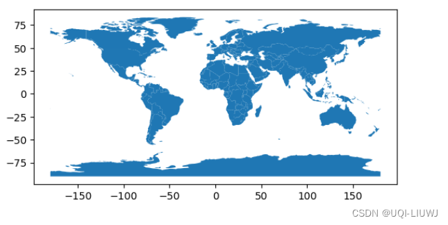

 1.2 column：根据geoDataFrame的哪一列来进行着色

world.plot(column='gdp_md_est')

 1.3 legend

给出颜色的图例

world.plot(column='gdp_md_est',
           legend=True)

 1.3.1 调整legend 相对于图的布局

from mpl_toolkits.axes_grid1 import make_axes_locatable
import matplotlib.pyplot as plt


fig, ax = plt.subplots(1, 1)
divider = make_axes_locatable(ax)
cax = divider.append_axes("right", size="5%", pad=0.1)


world.plot(column='pop_est', ax=ax, legend=True, cax=cax)

 1.3.2 legend_kwd 布局

world.plot(column='pop_est', 
           legend=True,
           legend_kwds={'label': "gdp_md_est",
                        'orientation': "horizontal"})

1.4 Cmap 颜色 

world.plot(column='pop_est', cmap='OrRd');

 

 1.5 boundary 绘制轮廓

world.boundary.plot()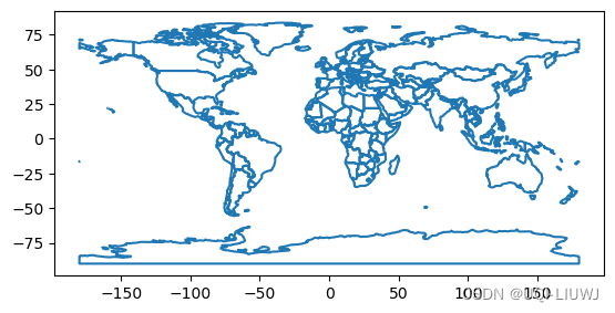

1.6 scheme 颜色映射的放缩方式

 可供选择的选项：“box_plot”、“equal_interval”、“fisher_jenks”、“fisher_jenks_sampled”、“headtail_breaks”、“jenks_caspall”、“jenks_caspall_forced”、“jenks_caspall_sampled”、“max_p_classifier”、“maximum_breaks”、“natural_breaks”、“quantiles”、“percentiles”、“std_mean”、“user_defined”

world.plot(column='pop_est',
           cmap='OrRd',
           scheme='quantiles')

 1.7 set_axis_off 不显示边框

world.plot(column='pop_est',
           cmap='OrRd',
           scheme='quantiles').set_axis_off()

 1.8 缺失值处理

1.8.1 构造缺失值

import numpy as np
world.loc[np.random.choice(world.index, 40), 'pop_est'] = np.nan
#选择40个区域，使其值变成nan

1.8.2 直接plot

会发现Nan的部分直接消失了

world.plot(column='pop_est');

1.8.3 missing_kwds

world.plot(column='pop_est', 
           missing_kwds={'color': 'lightgrey'});

 

 

world.plot(
    column="pop_est",
    missing_kwds={
        "color": "lightgrey",
        "edgecolor": "red",
        "hatch": "///"
    },
);

 2 在一种图上叠加另外一种图

2.0 另一个数据的导入

cities = gpd.read_file(gpd.datasets.get_path('naturalearth_cities'))
cities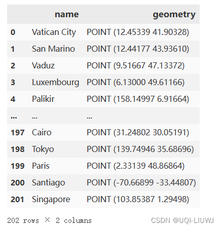

 

2.1 实现方法1：不使用matplotlib

ax=world.boundary.plot()
cities.plot(ax=ax,marker='*',color='red',markersize=10)

2.2 实现方法2：使用matplotlib

fig,ax=plt.subplots(1,1)

world.boundary.plot(ax=ax)
cities.plot(ax=ax,marker='*',color='red',markersize=10);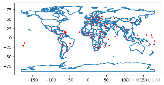

 

 3 绘制其他图

3.1 line——线图

world.plot(kind='line', x="pop_est")

 

3.2 bar——柱状图

world.plot(kind='bar', x="pop_est")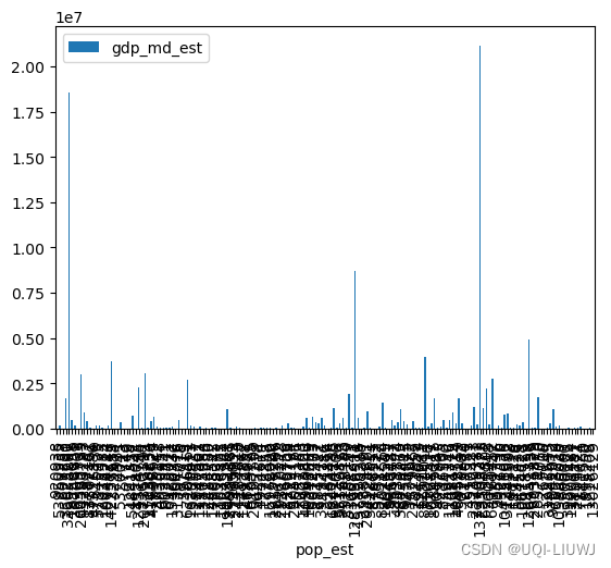

 

 3.3 hist——直方图

world.plot(kind='hist', x="pop_est")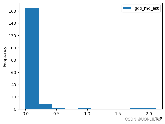

 3.4 box——箱式图

world.plot(kind='box', x="pop_est")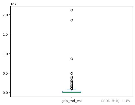

 

3.5 kde——密度图

world.plot(kind='kde', x="pop_est")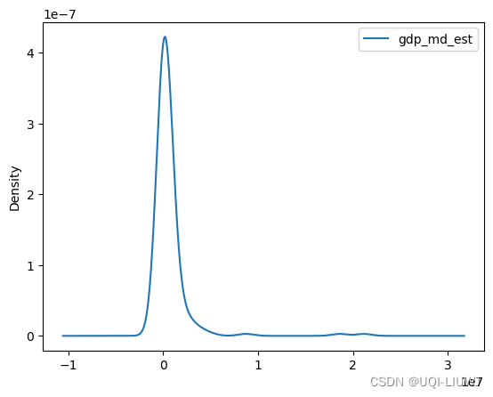

 

3.6 area——面积图

3.7 scatter——散点图

world.plot(kind='scatter', x="pop_est",y='gdp_md_est')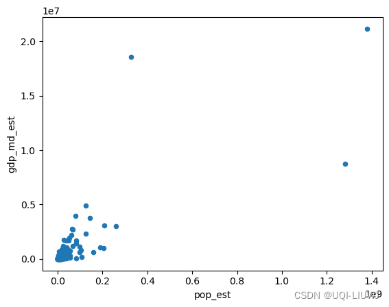

 

 

3.8 hexbin——六边形箱图

world.plot(kind='hexbin', x="pop_est",y='gdp_md_est')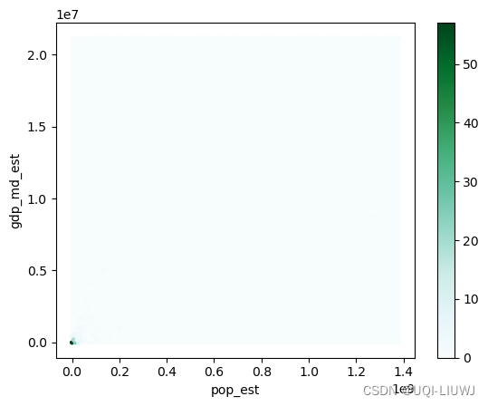

 

 

3.9 pie——饼图

world.plot(kind='pie', x="pop_est", y="gdp_md_est")