


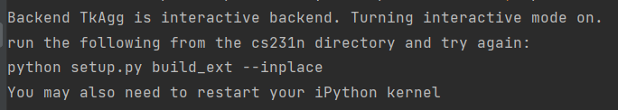
全神经网络
在前面的作业中,您在CIFAR-10上实现了一个完全连接的两层神经网络。实现是简单的,但不是非常模块化,因为损耗和梯度计算在一个单一的单片函数。对于一个简单的两层网络来说,这是可以管理的,但是当我们转向更大的模型时,这将变得不切实际。理想情况下,我们希望使用更模块化的设计来构建网络,这样我们就可以孤立地实现不同的层类型,然后将它们组合到具有不同架构的模型中。
在本练习中,我们将使用更模块化的方法实现全连接网络。对于每个层,我们将实现一个前向函数和一个后向函数。forward函数将接收输入、权重和其他参数,并返回一个输出和一个存储向后传递所需数据的缓存对象,如下所示:
前传递:
def layer_forward(x, w):
  """ Receive inputs x and weights w """
  # Do some computations ...
  z = # ... some intermediate value
  # Do some more computations ...
  out = # the output

  cache = (x, w, z, out) # Values we need to compute gradients

  return out, cache
后传递:
def layer_backward(dout, cache):
  """
  Receive dout (derivative of loss with respect to outputs) and cache,
  and compute derivative with respect to inputs.
  """
  # Unpack cache values
  x, w, z, out = cache

  # Use values in cache to compute derivatives
  dx = # Derivative of loss with respect to x
  dw = # Derivative of loss with respect to w

  return dx, dw
在以这种方式实现一堆层之后,我们将能够轻松地将它们组合起来,以构建具有不同体系结构的分类器。
除了实现任意深度的全连接网络,我们还将探索不同的优化更新规则,并引入Dropout作为正则化和Batch/Layer Normalization工具来更有效地优化深度网络。
还是跟之前类似
In[1]:
from __future__ import print_function
import time
import numpy as np
import matplotlib.pyplot as plt
from cs231n.classifiers.fc_net import *
from cs231n.data_utils import get_CIFAR10_data
from cs231n.gradient_check import eval_numerical_gradient, eval_numerical_gradient_array
from cs231n.solver import Solver

#%matplotlib inline
plt.rcParams['figure.figsize'] = (10.0, 8.0)
plt.rcParams['image.interpolation'] = 'nearest'
plt.rcParams['image.cmap'] = 'gray'

%load_ext autoreload
%autoreload 2

def rel_error(x, y):
  """ returns relative error """
  return np.max(np.abs(x - y) / (np.maximum(1e-8, np.abs(x) + np.abs(y))))
ln[2]:
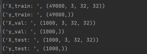
data = get_CIFAR10_data()
for k, v in list(data.items()):
  print(('%s: ' % k, v.shape))
ln[3]:
打开文件cs231n/layers.py并实现affine_forward函数
def affine_forward(x, w, b):
    """
    Computes the forward pass for an affine (fully-connected) layer.

    The input x has shape (N, d_1, ..., d_k) and contains a minibatch of N
    examples, where each example x[i] has shape (d_1, ..., d_k). We will
    reshape each input into a vector of dimension D = d_1 * ... * d_k, and
    then transform it to an output vector of dimension M.

    Inputs:
    - x: A numpy array containing input data, of shape (N, d_1, ..., d_k)
    - w: A numpy array of weights, of shape (D, M)
    - b: A numpy array of biases, of shape (M,)

    Returns a tuple of:
    - out: output, of shape (N, M)
    - cache: (x, w, b)
    """
    out = None
    ###########################################################################
    # TODO: Implement the affine forward pass. Store the result in out. You   #
    # will need to reshape the input into rows.                               #
    ###########################################################################
   	X = np.reshape(X, (X.shape[0], -1));
    out = X.dot(w) + b
    ###########################################################################
    #                             END OF YOUR CODE                            #
    ###########################################################################
    cache = (x, w, b)
    return out, cache
完成后测试你的实现:
ln[3]:
num_inputs = 2
input_shape = (4, 5, 6)
output_dim = 3
input_size = num_inputs * np.prod(input_shape)
weight_size = output_dim * np.prod(input_shape)
#numpy.linspace(start, stop, num)在指定的间隔内返回均匀间隔的数字。返回num均匀分布的样本,在[start, stop]。这个区间的端点可以任意的被排除在外
x = np.linspace(-0.1, 0.5, num=input_size).reshape(num_inputs, *input_shape)
w = np.linspace(-0.2, 0.3, num=weight_size).reshape(np.prod(input_shape), output_dim)
b = np.linspace(-0.3, 0.1, num=output_dim)
out, _ = affine_forward(x, w, b)
correct_out = np.array([[ 1.49834967, 1.70660132, 1.91485297],
[ 3.25553199, 3.5141327, 3.77273342]])
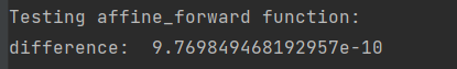
# Compare your output with ours. The error should be around e-9 or less.
print('Testing affine_forward function:')
print('difference: ', rel_error(out, correct_out))
现在实现affine_backward函数,并使用数值梯度检查测试您的实现。
def affine_backward(dout, cache):
    """
    Computes the backward pass for an affine layer.

    Inputs:
    - dout: Upstream derivative, of shape (N, M)
    - cache: Tuple of:
      - x: Input data, of shape (N, d_1, ... d_k)
      - w: Weights, of shape (D, M)
      - b: Biases, of shape (M,)

    Returns a tuple of:
    - dx: Gradient with respect to x, of shape (N, d1, ..., d_k)
    - dw: Gradient with respect to w, of shape (D, M)
    - db: Gradient with respect to b, of shape (M,)
    """
    x, w, b = cache
    dx, dw, db = None, None, None
    ###########################################################################
    # TODO: Implement the affine backward pass.                               #
    ###########################################################################
    dim_shape = np.prod(x[0].shape)
    N = x.shape[0]
    X = x.reshape(N, dim_shape)
    # input gradient
    dx = dout.dot(w.T)
    dx = dx.reshape(x.shape)
    # weight gradient
    dw = X.T.dot(dout)
    # bias gradient
    db = dout.sum(axis=0)
    ###########################################################################
    #                             END OF YOUR CODE                            #
    ###########################################################################
    return dx, dw, db
测试:
ln[4]:
np.random.seed(231)
x = np.random.randn(10, 2, 3)
w = np.random.randn(6, 5)
b = np.random.randn(5)
dout = np.random.randn(10, 5)
dx_num = eval_numerical_gradient_array(lambda x: affine_forward(x, w, b)[0], x, dout)
dw_num = eval_numerical_gradient_array(lambda w: affine_forward(x, w, b)[0], w, dout)
db_num = eval_numerical_gradient_array(lambda b: affine_forward(x, w, b)[0], b, dout)
_, cache = affine_forward(x, w, b)
dx, dw, db = affine_backward(dout, cache)
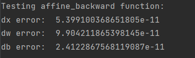
# The error should be around e-10 or less
print('Testing affine_backward function:')
print('dx error: ', rel_error(dx_num, dx))
print('dw error: ', rel_error(dw_num, dw))
print('db error: ', rel_error(db_num, db))
在relu_forward函数中实现ReLU激活函数的forward pass函数
回顾一下ReLU:

def relu_forward(x):
    """
    Computes the forward pass for a layer of rectified linear units (ReLUs).

    Input:
    - x: Inputs, of any shape

    Returns a tuple of:
    - out: Output, of the same shape as x
    - cache: x
    """
    out = None
    ###########################################################################
    # TODO: Implement the ReLU forward pass.                                  #
    ###########################################################################
    out = np.maximum(0, x)
    ###########################################################################
    #                             END OF YOUR CODE                            #
    ###########################################################################
    cache = x
    return out, cache
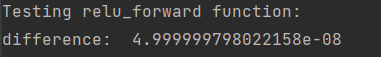
测试你的实现:
ln[5]:
x = np.linspace(-0.5, 0.5, num=12).reshape(3, 4)

out, _ = relu_forward(x)
correct_out = np.array([[ 0.,          0.,          0.,          0.,        ],
                        [ 0.,          0.,          0.04545455,  0.13636364,],
                        [ 0.22727273,  0.31818182,  0.40909091,  0.5,       ]])

# Compare your output with ours. The error should be on the order of e-8
print('Testing relu_forward function:')
print('difference: ', rel_error(out, correct_out))
在relu_backward函数中实现ReLU激活函数的backward pass:
def relu_backward(dout, cache):
    """
    Computes the backward pass for a layer of rectified linear units (ReLUs).

    Input:
    - dout: Upstream derivatives, of any shape
    - cache: Input x, of same shape as dout

    Returns:
    - dx: Gradient with respect to x
    """
    dx, x = None, cache
    ###########################################################################
    # TODO: Implement the ReLU backward pass.                                 #
    ###########################################################################
    dx = dout * (x > 0)
    ###########################################################################
    #                             END OF YOUR CODE                            #
    ###########################################################################
    return dx
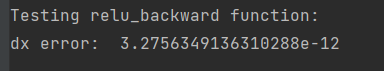
测试你的实现
ln[6]:
np.random.seed(231)
x = np.random.randn(10, 10)
dout = np.random.randn(*x.shape)

dx_num = eval_numerical_gradient_array(lambda x: relu_forward(x)[0], x, dout)

_, cache = relu_forward(x)
dx = relu_backward(dout, cache)

# The error should be on the order of e-12
print('Testing relu_backward function:')
print('dx error: ', rel_error(dx_num, dx))
内联问题1:
我们只要求你实现ReLU,但是有很多不同的激活函数神经网络可以使用,每个都有各自的优点和缺点。具有激活功能的一个常见问题是零(或接近于零)梯度流在反向传播。下面哪个激活函数有这个问题?如果你考虑一维情况下的这些函数,什么类型的输入会导致这种行为?
1.Sigmoid
2.ReLU
3.Leaky ReLU
答:
1.Sigmoid函数受到梯度消失问题的困扰,因为梯度在函数尾部取小值(接近0)。
2.ReLU的梯度是0或1。因此当所有的输入值都为负时,它可能会遭受梯度消失的问题。然而,拥有所有负面输入的可能性较小。因为这个问题只发生在一个方面(负值),一些神经元永远不会更新,即它们将“死亡”。一个可以使梯度消失的一维例子是只考虑负值,比如[-1,-2,-4,-5]
3.Leaky ReLU试图解决“死亡”神经元的ReLU问题,当我们有负值时,考虑小的负斜率,即,如果x < 0,then alpha,else x,其中alpha可以等于0.01。一个可以使梯度消失的一维例子是考虑所有的零值,例如,[0,0,0,0],它只会在网络初始化不好的情况下发生。
下面是这些函数的图

"三明治层’
在神经网络中有一些常见的层模式。affine layers are frequently followed by a ReLU nonlinearity。为了简化这些常见模式,我们在文件cs231n/layer_utils.py中定义了几个方便的层。
现在看一下affine_relu_forward和affine_relu_backward函数,并运行下面的数值梯度检查向后传递:
def affine_relu_forward(x, w, b):
    """
    Convenience layer that performs an affine transform followed by a ReLU

    Inputs:
    - x: Input to the affine layer
    - w, b: Weights for the affine layer

    Returns a tuple of:
    - out: Output from the ReLU
    - cache: Object to give to the backward pass
    """
    a, fc_cache = affine_forward(x, w, b)
    out, relu_cache = relu_forward(a)
    cache = (fc_cache, relu_cache)
    return out, cache


def affine_relu_backward(dout, cache):
    """
    Backward pass for the affine-relu convenience layer
    """
    fc_cache, relu_cache = cache
    da = relu_backward(dout, relu_cache)
    dx, dw, db = affine_backward(da, fc_cache)
    return dx, dw, db
In[7]:
from cs231n.layer_utils import affine_relu_forward, affine_relu_backward
np.random.seed(231)
x = np.random.randn(2, 3, 4)
w = np.random.randn(12, 10)
b = np.random.randn(10)
dout = np.random.randn(2, 10)
out, cache = affine_relu_forward(x, w, b)
dx, dw, db = affine_relu_backward(dout, cache)
dx_num = eval_numerical_gradient_array(lambda x: affine_relu_forward(x, w, b)[0], x, dout)
dw_num = eval_numerical_gradient_array(lambda w: affine_relu_forward(x, w, b)[0], w, dout)
db_num = eval_numerical_gradient_array(lambda b: affine_relu_forward(x, w, b)[0], b, dout)
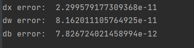
# Relative error should be around e-10 or less
print('Testing affine_relu_forward and affine_relu_backward:')
print('dx error: ', rel_error(dx_num, dx))
print('dw error: ', rel_error(dw_num, dw))
print('db error: ', rel_error(db_num, db))
损失层:
softmax vs svm
In[8]:
np.random.seed(231)
num_classes, num_inputs = 10, 50
x = 0.001 * np.random.randn(num_inputs, num_classes)
y = np.random.randint(num_classes, size=num_inputs)
dx_num = eval_numerical_gradient(lambda x: svm_loss(x, y)[0], x, verbose=False)
loss, dx = svm_loss(x, y)
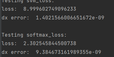
# Test svm_loss function. Loss should be around 9 and dx error should be around the order of e-9
print('Testing svm_loss:')
print('loss: ', loss)
print('dx error: ', rel_error(dx_num, dx))
dx_num = eval_numerical_gradient(lambda x: softmax_loss(x, y)[0], x, verbose=False)
loss, dx = softmax_loss(x, y)
# Test softmax_loss function. Loss should be close to 2.3 and dx error should be around e-8
print('\nTesting softmax_loss:')
print('loss: ', loss)
print('dx error: ', rel_error(dx_num, dx))
Two-layer Network
打开文件cs231n/classifiers/fc_net.py,完成TwoLayerNet类的实现
结构:affine - relu - affine - softmax
初始化:
class TwoLayerNet(object):
    """
    A two-layer fully-connected neural network with ReLU nonlinearity and
    softmax loss that uses a modular layer design. We assume an input dimension
    of D, a hidden dimension of H, and perform classification over C classes.

    The architecture should be affine - relu - affine - softmax.

    Note that this class does not implement gradient descent; instead, it
    will interact with a separate Solver object that is responsible for running
    optimization.

    The learnable parameters of the model are stored in the dictionary
    self.params that maps parameter names to numpy arrays.
    """

    def __init__(self, input_dim=3*32*32, hidden_dim=100, num_classes=10,
                 weight_scale=1e-3, reg=0.0):
        """
        Initialize a new network.

        Inputs:
        - input_dim: An integer giving the size of the input
        - hidden_dim: An integer giving the size of the hidden layer
        - num_classes: An integer giving the number of classes to classify
        - weight_scale: Scalar giving the standard deviation for random
          initialization of the weights.
        - reg: Scalar giving L2 regularization strength.
        """
        self.params = {}
        self.reg = reg

        ############################################################################
        # TODO: Initialize the weights and biases of the two-layer net. Weights    #
        # should be initialized from a Gaussian centered at 0.0 with               #
        # standard deviation equal to weight_scale, and biases should be           #
        # initialized to zero. All weights and biases should be stored in the      #
        # dictionary self.params, with first layer weights                         #
        # and biases using the keys 'W1' and 'b1' and second layer                 #
        # weights and biases using the keys 'W2' and 'b2'.                         #
        ############################################################################
        self.params['W1'] = weight_scale * np.random.randn(input_dim, hidden_dim)
        self.params['W2'] = weight_scale * np.random.randn(hidden_dim, num_classes)
        self.params['b1'] = np.zeros(hidden_dim)
        self.params['b2'] = np.zeros(num_classes)
        ############################################################################
        #                             END OF YOUR CODE                             #
        ############################################################################
损失函数:
    def loss(self, X, y=None):
        """
        Compute loss and gradient for a minibatch of data.

        Inputs:
        - X: Array of input data of shape (N, d_1, ..., d_k)
        - y: Array of labels, of shape (N,). y[i] gives the label for X[i].

        Returns:
        If y is None, then run a test-time forward pass of the model and return:
        - scores: Array of shape (N, C) giving classification scores, where
          scores[i, c] is the classification score for X[i] and class c.

        If y is not None, then run a training-time forward and backward pass and
        return a tuple of:
        - loss: Scalar value giving the loss
        - grads: Dictionary with the same keys as self.params, mapping parameter
          names to gradients of the loss with respect to those parameters.
        """
        scores = None
        W1 = self.params['W1']
        W2 = self.params['W2']
        b1 = self.params['b1']
        b2 = self.params['b2']
        ############################################################################
        # TODO: Implement the forward pass for the two-layer net, computing the    #
        # class scores for X and storing them in the scores variable.              #
        ############################################################################
        X2, relu_cache = affine_relu_forward(X, W1, b1)
        scores, relu2_cache = affine_relu_forward(X2, W2, b2)
        ############################################################################
        #                             END OF YOUR CODE                             #
        ############################################################################

        # If y is None then we are in test mode so just return scores
        if y is None:
            return scores

        loss, grads = 0, {}
        ############################################################################
        # TODO: Implement the backward pass for the two-layer net. Store the loss  #
        # in the loss variable and gradients in the grads dictionary. Compute data #
        # loss using softmax, and make sure that grads[k] holds the gradients for  #
        # self.params[k]. Don't forget to add L2 regularization!                   #
        #                                                                          #
        # NOTE: To ensure that your implementation matches ours and you pass the   #
        # automated tests, make sure that your L2 regularization includes a factor #
        # of 0.5 to simplify the expression for the gradient.                      #
        ############################################################################
        # calculate loss
        loss, softmax_grad = softmax_loss(scores, y)
        loss += 0.5 * self.reg * ( np.sum(W1 * W1) + np.sum(W2 * W2) )

        # calculate gradient
        dx2, dw2, db2 = affine_relu_backward(softmax_grad, relu2_cache)
        dx, dw, db = affine_relu_backward(dx2, relu_cache)
        grads['W2'] = dw2 + self.reg * W2
        grads['b2'] = db2
        grads['W1'] = dw + self.reg * W1
        grads['b1'] = db
        ############################################################################
        #                             END OF YOUR CODE                             #
        ############################################################################

        return loss, grads
ln[9]:
np.random.seed(231)
N, D, H, C = 3, 5, 50, 7
X = np.random.randn(N, D)
y = np.random.randint(C, size=N)

std = 1e-3
model = TwoLayerNet(input_dim=D, hidden_dim=H, num_classes=C, weight_scale=std)

print('Testing initialization ... ')
W1_std = abs(model.params['W1'].std() - std)
b1 = model.params['b1']
W2_std = abs(model.params['W2'].std() - std)
b2 = model.params['b2']
assert W1_std < std / 10, 'First layer weights do not seem right'
assert np.all(b1 == 0), 'First layer biases do not seem right'
assert W2_std < std / 10, 'Second layer weights do not seem right'
assert np.all(b2 == 0), 'Second layer biases do not seem right'

print('Testing test-time forward pass ... ')
model.params['W1'] = np.linspace(-0.7, 0.3, num=D*H).reshape(D, H)
model.params['b1'] = np.linspace(-0.1, 0.9, num=H)
model.params['W2'] = np.linspace(-0.3, 0.4, num=H*C).reshape(H, C)
model.params['b2'] = np.linspace(-0.9, 0.1, num=C)
X = np.linspace(-5.5, 4.5, num=N*D).reshape(D, N).T
scores = model.loss(X)
correct_scores = np.asarray(
  [[11.53165108,  12.2917344,   13.05181771,  13.81190102,  14.57198434, 15.33206765,  16.09215096],
   [12.05769098,  12.74614105,  13.43459113,  14.1230412,   14.81149128, 15.49994135,  16.18839143],
   [12.58373087,  13.20054771,  13.81736455,  14.43418138,  15.05099822, 15.66781506,  16.2846319 ]])
scores_diff = np.abs(scores - correct_scores).sum()
assert scores_diff < 1e-6, 'Problem with test-time forward pass'

print('Testing training loss (no regularization)')
y = np.asarray([0, 5, 1])
loss, grads = model.loss(X, y)
correct_loss = 3.4702243556
assert abs(loss - correct_loss) < 1e-10, 'Problem with training-time loss'

model.reg = 1.0
loss, grads = model.loss(X, y)
correct_loss = 26.5948426952
assert abs(loss - correct_loss) < 1e-10, 'Problem with regularization loss'

# Errors should be around e-7 or less
for reg in [0.0, 0.7]:
  print('Running numeric gradient check with reg = ', reg)
  model.reg = reg
  loss, grads = model.loss(X, y)

  for name in sorted(grads):
    f = lambda _: model.loss(X, y)[0]
    grad_num = eval_numerical_gradient(f, model.params[name], verbose=False)
    print('%s relative error: %.2e' % (name, rel_error(grad_num, grads[name])))

Solver
在上一个任务中,训练模型的逻辑被耦合到模型本身。按照一个更模块化的设计,在这个作业中,我们将训练模型的逻辑拆分为一个单独的类。
打开文件cs231n/solver.py并通读它以熟悉该API。在这样做之后,使用一个求解器实例来训练TwoLayerNet,使其在验证集上达到至少50%的精度。

In[10]:
model = TwoLayerNet()
solver = None
best_val = -1
##############################################################################
# TODO: Use a Solver instance to train a TwoLayerNet that achieves at least #
# 50% accuracy on the validation set. #
##############################################################################
# Generate random hyperparameters given ranges for each of them
def generate_random_hyperparams(lr_min, lr_max, reg_min, reg_max, h_min, h_max):
#np.random.uniform从一个均匀分布[low,high)中随机采样,注意定义域是左闭右开,即包含low,不包含high
lr = 10**np.random.uniform(lr_min,lr_max)
reg = 10**np.random.uniform(reg_min,reg_max)
hidden = np.random.randint(h_min, h_max)
return lr, reg, hidden
for i in range(20):
lr, reg, hidden_size = generate_random_hyperparams(-4,-2, -7, -4, 10, 200)
model = TwoLayerNet(hidden_dim = hidden_size, reg= reg)
cur_solver = Solver(model, data, update_rule='sgd', optim_config={'learning_rate':lr},
lr_decay=0.95, num_epochs=5,batch_size=200, print_every=-1)
cur_solver.train()
val_accuracy = cur_solver.best_val_acc
if best_val < val_accuracy:
best_val = val_accuracy
best_lr = lr
best_reg = reg
best_hi = hidden_size
solver = cur_solver
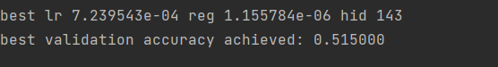
print('best lr %e reg %e hid %d' % (best_lr,best_reg,best_hi))
print('best validation accuracy achieved: %f' % best_val)
##############################################################################
# END OF YOUR CODE #
##############################################################################
可视化loss和accuracy:
ln[11]:
plt.subplot(2, 1, 1)
plt.title('Training loss')
plt.plot(solver.loss_history, 'o')
plt.xlabel('Iteration')

plt.subplot(2, 1, 2)
plt.title('Accuracy')
plt.plot(solver.train_acc_history, '-o', label='train')
plt.plot(solver.val_acc_history, '-o', label='val')
plt.plot([0.5] * len(solver.val_acc_history), 'k--')
plt.xlabel('Epoch')
plt.legend(loc='lower right')
plt.gcf().set_size_inches(15, 12)
plt.show()

多层网络
接下来,您将实现一个具有任意数量隐藏层的完全连接的网络。
阅读文件cs231n/classifiers/fc_net.py中的fulllyconnectednet类。
实现初始化、向前传递和向后传递。暂时不要担心实现dropout或batch/layer规范化;我们将很快添加这些功能。
初始损耗和梯度检查
作为一个完整性检查,运行以下命令检查初始损失,并在有和没有正则化的情况下检查网络的梯度。最初的损失看起来合理吗?
对于梯度检查,您应该期望看到大约1e-7或更少的错误。
class FullyConnectedNet(object):
    """
    A fully-connected neural network with an arbitrary number of hidden layers,
    ReLU nonlinearities, and a softmax loss function. This will also implement
    dropout and batch/layer normalization as options. For a network with L layers,
    the architecture will be

    {affine - [batch/layer norm] - relu - [dropout]} x (L - 1) - affine - softmax

    where batch/layer normalization and dropout are optional, and the {...} block is
    repeated L - 1 times.

    Similar to the TwoLayerNet above, learnable parameters are stored in the
    self.params dictionary and will be learned using the Solver class.
    """

    def __init__(self, hidden_dims, input_dim=3*32*32, num_classes=10,
                 dropout=1, normalization=None, reg=0.0,
                 weight_scale=1e-2, dtype=np.float32, seed=None):
        """
        Initialize a new FullyConnectedNet.

        Inputs:
        - hidden_dims: A list of integers giving the size of each hidden layer.
        - input_dim: An integer giving the size of the input.
        - num_classes: An integer giving the number of classes to classify.
        - dropout: Scalar between 0 and 1 giving dropout strength. If dropout=1 then
          the network should not use dropout at all.
        - normalization: What type of normalization the network should use. Valid values
          are "batchnorm", "layernorm", or None for no normalization (the default).
        - reg: Scalar giving L2 regularization strength.
        - weight_scale: Scalar giving the standard deviation for random
          initialization of the weights.
        - dtype: A numpy datatype object; all computations will be performed using
          this datatype. float32 is faster but less accurate, so you should use
          float64 for numeric gradient checking.
        - seed: If not None, then pass this random seed to the dropout layers. This
          will make the dropout layers deteriminstic so we can gradient check the
          model.
        """
        self.normalization = normalization
        self.use_dropout = dropout != 1
        self.reg = reg
        self.num_layers = 1 + len(hidden_dims)
        self.dtype = dtype
        self.params = {}

        ############################################################################
        # TODO: Initialize the parameters of the network, storing all values in    #
        # the self.params dictionary. Store weights and biases for the first layer #
        # in W1 and b1; for the second layer use W2 and b2, etc. Weights should be #
        # initialized from a normal distribution centered at 0 with standard       #
        # deviation equal to weight_scale. Biases should be initialized to zero.   #
        #                                                                          #
        # When using batch normalization, store scale and shift parameters for the #
        # first layer in gamma1 and beta1; for the second layer use gamma2 and     #
        # beta2, etc. Scale parameters should be initialized to ones and shift     #
        # parameters should be initialized to zeros.                               #
        ############################################################################
        layers_dims = np.hstack([input_dim, hidden_dims, num_classes])
        for i in range(self.num_layers):
            self.params['W'+str(i+1)] = weight_scale*np.random.randn(layers_dims[i],layers_dims[i+1])
            self.params['b'+str(i+1)] = np.zeros(layers_dims[i+1])

        if self.normalization != None:
            # batch/layer norm parameters
            for i in range(self.num_layers-1):
                self.params['gamma'+str(i+1)] = np.ones(layers_dims[i+1])
                self.params['beta' +str(i+1)] = np.zeros(layers_dims[i+1])
        ############################################################################
        #                             END OF YOUR CODE                             #
        ############################################################################

        # When using dropout we need to pass a dropout_param dictionary to each
        # dropout layer so that the layer knows the dropout probability and the mode
        # (train / test). You can pass the same dropout_param to each dropout layer.
        self.dropout_param = {}
        if self.use_dropout:
            self.dropout_param = {'mode': 'train', 'p': dropout}
            if seed is not None:
                self.dropout_param['seed'] = seed

        # With batch normalization we need to keep track of running means and
        # variances, so we need to pass a special bn_param object to each batch
        # normalization layer. You should pass self.bn_params[0] to the forward pass
        # of the first batch normalization layer, self.bn_params[1] to the forward
        # pass of the second batch normalization layer, etc.
        self.bn_params = []
        if self.normalization=='batchnorm':
            self.bn_params = [{'mode': 'train'} for i in range(self.num_layers - 1)]
        if self.normalization=='layernorm':
            self.bn_params = [{} for i in range(self.num_layers - 1)]

        # Cast all parameters to the correct datatype
        for k, v in self.params.items():
            self.params[k] = v.astype(dtype)


    def loss(self, X, y=None):
        """
        Compute loss and gradient for the fully-connected net.

        Input / output: Same as TwoLayerNet above.
        """
        X = X.astype(self.dtype)
        mode = 'test' if y is None else 'train'

        # Set train/test mode for batchnorm params and dropout param since they
        # behave differently during training and testing.
        if self.use_dropout:
            self.dropout_param['mode'] = mode
        if self.normalization=='batchnorm':
            for bn_param in self.bn_params:
                bn_param['mode'] = mode
        scores = None
        ############################################################################
        # TODO: Implement the forward pass for the fully-connected net, computing  #
        # the class scores for X and storing them in the scores variable.          #
        #                                                                          #
        # When using dropout, you'll need to pass self.dropout_param to each       #
        # dropout forward pass.                                                    #
        #                                                                          #
        # When using batch normalization, you'll need to pass self.bn_params[0] to #
        # the forward pass for the first batch normalization layer, pass           #
        # self.bn_params[1] to the forward pass for the second batch normalization #
        # layer, etc.                                                              #
        ############################################################################
        x = X
        caches = []
        gamma, beta, bn_params = None, None, None
        for i in range(self.num_layers-1):
            w = self.params['W'+str(i+1)]
            b = self.params['b'+str(i+1)]
            if self.normalization != None:
               gamma = self.params['gamma'+str(i+1)]
               beta  = self.params['beta'+str(i+1)]
               bn_params = self.bn_params[i]
            x, cache = affine_norm_relu_forward(x,w,b, gamma, beta, bn_params, self.normalization,
                                                self.use_dropout, self.dropout_param)
            caches.append(cache)
        w = self.params['W'+str(self.num_layers)]
        b = self.params['b'+str(self.num_layers)]
        scores, cache = affine_forward(x,w,b)
        caches.append(cache)
        ############################################################################
        #                             END OF YOUR CODE                             #
        ############################################################################

        # If test mode return early
        if mode == 'test':
            return scores

        loss, grads = 0.0, {}
        ############################################################################
        # TODO: Implement the backward pass for the fully-connected net. Store the #
        # loss in the loss variable and gradients in the grads dictionary. Compute #
        # data loss using softmax, and make sure that grads[k] holds the gradients #
        # for self.params[k]. Don't forget to add L2 regularization!               #
        #                                                                          #
        # When using batch/layer normalization, you don't need to regularize the   #
        # scale and shift parameters.                                              #
        #                                                                          #
        # NOTE: To ensure that your implementation matches ours and you pass the   #
        # automated tests, make sure that your L2 regularization includes a factor #
        # of 0.5 to simplify the expression for the gradient.                      #
        ############################################################################
        # calculate loss
        loss, softmax_grad = softmax_loss(scores, y)
        for i in range(self.num_layers):
            w = self.params['W'+str(i+1)]
            loss += 0.5 * self.reg * np.sum(w * w)

        # calculate gradients
        dout = softmax_grad
        dout, dw, db = affine_backward(dout, caches[self.num_layers - 1])
        grads['W' + str(self.num_layers)] = dw + self.reg * self.params['W' + str(self.num_layers)]
        grads['b' + str(self.num_layers)] = db

        for i in range(self.num_layers - 2, -1, -1):
            dx, dw, db, dgamma, dbeta = affine_norm_relu_backward(dout, caches[i], self.normalization,
                                                                  self.use_dropout)
            if self.normalization != None:
               grads['gamma'+str(i+1)] = dgamma
               grads['beta' +str(i+1)] = dbeta
            grads['W' + str(i + 1)] = dw + self.reg * self.params['W' + str(i + 1)]
            grads['b' + str(i + 1)] = db
            dout = dx
        ############################################################################
        #                             END OF YOUR CODE                             #
        ############################################################################

        return loss, grads
ln[12]:
np.random.seed(231)
N, D, H1, H2, C = 2, 15, 20, 30, 10
X = np.random.randn(N, D)
y = np.random.randint(C, size=(N,))

for reg in [0, 3.14]:
  print('Running check with reg = ', reg)
  model = FullyConnectedNet([H1, H2], input_dim=D, num_classes=C,
                            reg=reg, weight_scale=5e-2, dtype=np.float64)

  loss, grads = model.loss(X, y)
  print('Initial loss: ', loss)

  # Most of the errors should be on the order of e-7 or smaller.
  # NOTE: It is fine however to see an error for W2 on the order of e-5
  # for the check when reg = 0.0
  for name in sorted(grads):
    f = lambda _: model.loss(X, y)[0]
    grad_num = eval_numerical_gradient(f, model.params[name], verbose=False, h=1e-5)
    print('%s relative error: %.2e' % (name, rel_error(grad_num, grads[name])))

作为另一个完整性检查,请确保您可以过拟合一个包含50张图片的小数据集。首先,我们将尝试一个三层网络,每个隐含层有100个单元。在接下来的单元格中,调整学习率和初始化规模,使其过拟合,并在20个epoch内达到100%的训练精度。
ln[13]:
num_train = 50
small_data = {
  'X_train': data['X_train'][:num_train],
  'y_train': data['y_train'][:num_train],
  'X_val': data['X_val'],
  'y_val': data['y_val'],
}

# Obtained with random search
weight_scale = 2e-2
learning_rate = 3e-3

model = FullyConnectedNet([100, 100],
              weight_scale=weight_scale, dtype=np.float64)
solver = Solver(model, small_data,
                print_every=10, num_epochs=20, batch_size=25,
                update_rule='sgd',
                optim_config={
                  'learning_rate': learning_rate,
                }
         )
solver.train()

plt.plot(solver.loss_history, 'o')
plt.title('Training loss history')
plt.xlabel('Iteration')
plt.ylabel('Training loss')
plt.show()

现在尝试使用五层网络,每层100个单元来过拟合50个训练示例。再次,您将不得不调整学习率和权重初始化,但您应该能够在20个epoch内实现100%的训练准确性。
num_train = 50
small_data = {
  'X_train': data['X_train'][:num_train],
  'y_train': data['y_train'][:num_train],
  'X_val': data['X_val'],
  'y_val': data['y_val'],
}

# Obtained with random search
learning_rate = 2e-3
weight_scale = 9e-2

model = FullyConnectedNet([100, 100, 100, 100],
                weight_scale=weight_scale, dtype=np.float64)
solver = Solver(model, small_data,
                print_every=10, num_epochs=20, batch_size=25,
                update_rule='sgd',
                optim_config={
                  'learning_rate': learning_rate,
                }
         )
solver.train()

plt.plot(solver.loss_history, 'o')
plt.title('Training loss history')
plt.xlabel('Iteration')
plt.ylabel('Training loss')
plt.show()

内联问题2:
对比训练三层网络和训练五层网络的相对难度?特别是,根据您的经验,哪个网络似乎对初始化规模更敏感?你认为为什么会这样呢?
答:
对比两种网络的训练难度,五层网络对初始化规模更敏感。在我看来,这是由于层数。当我们有一个更深的网络时,设置一个小的规模会导致梯度的消失,另一方面,设置一个大的规模会导致梯度的爆炸,在更深的网络中,这种情况发生的频率比在浅层网络中更高。找到一个正确的规模比三层网络更难,但可以通过随机搜索得到。我们可以在下一个例子中看到这种行为:
ln[15]:
num_train = 50
small_data = {
  'X_train': data['X_train'][:num_train],
  'y_train': data['y_train'][:num_train],
  'X_val': data['X_val'],
  'y_val': data['y_val'],
}

np.random.seed(1)
learning_rate = 1e-2
weight_scale = [1e-5, 1e-3, 1e-2, 5e-2, 1e-1, 5e-1]

for we in weight_scale:
    model = FullyConnectedNet([100,100,100,100],
                    weight_scale=we, dtype=np.float64)
    solver = Solver(model, small_data,
                    print_every=-1, num_epochs=20, batch_size=25,
                    update_rule='sgd',
                    optim_config={
                      'learning_rate': learning_rate,
                    }, verbose = False
             )
    solver.train()
    train_accuracy = solver.train_acc_history[len(solver.train_acc_history) - 1]
    print("learning_rate=%lf, weight_scale=%lf, train_accuracy=%lf" % (learning_rate, we, train_accuracy))
    for k,v in sorted(model.params.items()):
        if k[0] == 'W': #only print weights
            print("%s - mean=%lf, std=%lf" % (k, v.mean(), v.std()))
    print()
如前所述,当使用较小的权重尺度(消失梯度)时,参数的均值和标准差接近于零,增加尺度可以改善这些值;然而,增加太多会导致较大的值(爆炸式梯度)。当将隐藏层的大小更改为两个时,这个问题也会出现。然而,不同于五层网络的特殊权重w(5e-2),权重尺度更容易找到(1e-2)。注意,这些权重值取决于学习率。
这里的结果我就不贴了,太高直接报错了。。。
更新规则
到目前为止,我们使用普通的随机梯度下降(SGD)作为我们的更新规则。更复杂的更新规则可以让训练深度网络变得更容易。我们将实现一些最常用的更新规则,并将它们与普通的SGD进行比较。
SGD +动量
带动量的随机梯度下降是一种应用广泛的更新规则,它比普通的随机梯度下降更容易使深度网络收敛。


打开文件cs231n/opt .py并阅读该文件顶部的文档,以确保您理解了API。在函数sgd_momentum中实现SGD+momentum更新规则,并运行以下命令检查您的实现。您应该看到小于e-8的错误。
def sgd_momentum(w, dw, config=None):
    """
    Performs stochastic gradient descent with momentum.

    config format:
    - learning_rate: Scalar learning rate.
    - momentum: Scalar between 0 and 1 giving the momentum value.
      Setting momentum = 0 reduces to sgd.
    - velocity: A numpy array of the same shape as w and dw used to store a
      moving average of the gradients.
    """
    if config is None: config = {}
    config.setdefault('learning_rate', 1e-2)
    config.setdefault('momentum', 0.9)
    v = config.get('velocity', np.zeros_like(w))

    next_w = None
    ###########################################################################
    # TODO: Implement the momentum update formula. Store the updated value in #
    # the next_w variable. You should also use and update the velocity v.     #
    ###########################################################################
    v = config['momentum'] * v - config['learning_rate'] * dw
    next_w = w + v
    ###########################################################################
    #                             END OF YOUR CODE                            #
    ###########################################################################
    config['velocity'] = v

    return next_w, config
ln[16]:
from cs231n.optim import sgd_momentum
N, D = 4, 5
w = np.linspace(-0.4, 0.6, num=N*D).reshape(N, D)
dw = np.linspace(-0.6, 0.4, num=N*D).reshape(N, D)
v = np.linspace(0.6, 0.9, num=N*D).reshape(N, D)
config = {'learning_rate': 1e-3, 'velocity': v}
next_w, _ = sgd_momentum(w, dw, config=config)
expected_next_w = np.asarray([
[ 0.1406, 0.20738947, 0.27417895, 0.34096842, 0.40775789],
[ 0.47454737, 0.54133684, 0.60812632, 0.67491579, 0.74170526],
[ 0.80849474, 0.87528421, 0.94207368, 1.00886316, 1.07565263],
[ 1.14244211, 1.20923158, 1.27602105, 1.34281053, 1.4096 ]])
expected_velocity = np.asarray([
[ 0.5406, 0.55475789, 0.56891579, 0.58307368, 0.59723158],
[ 0.61138947, 0.62554737, 0.63970526, 0.65386316, 0.66802105],
[ 0.68217895, 0.69633684, 0.71049474, 0.72465263, 0.73881053],
[ 0.75296842, 0.76712632, 0.78128421, 0.79544211, 0.8096 ]])
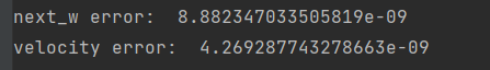
# Should see relative errors around e-8 or less
print('next_w error: ', rel_error(next_w, expected_next_w))
print('velocity error: ', rel_error(expected_velocity, config['velocity']))
一旦你这样做了,运行下面的方法来训练一个包含SGD和SGD+动量的六层网络。你应该看到SGD+动量更新规则收敛得更快了。
ln[17]:
num_train = 4000
small_data = {
  'X_train': data['X_train'][:num_train],
  'y_train': data['y_train'][:num_train],
  'X_val': data['X_val'],
  'y_val': data['y_val'],
}

solvers = {}

for update_rule in ['sgd', 'sgd_momentum']:
  print('running with ', update_rule)
  model = FullyConnectedNet([100, 100, 100, 100, 100], weight_scale=5e-2)

  solver = Solver(model, small_data,
                  num_epochs=5, batch_size=100,
                  update_rule=update_rule,
                  optim_config={
                    'learning_rate': 1e-2,
                  },
                  verbose=True)
  solvers[update_rule] = solver
  solver.train()
  print()

plt.subplot(3, 1, 1)
plt.title('Training loss')
plt.xlabel('Iteration')

plt.subplot(3, 1, 2)
plt.title('Training accuracy')
plt.xlabel('Epoch')

plt.subplot(3, 1, 3)
plt.title('Validation accuracy')
plt.xlabel('Epoch')

for update_rule, solver in list(solvers.items()):
  plt.subplot(3, 1, 1)
  plt.plot(solver.loss_history, 'o', label=update_rule)

  plt.subplot(3, 1, 2)
  plt.plot(solver.train_acc_history, '-o', label=update_rule)

  plt.subplot(3, 1, 3)
  plt.plot(solver.val_acc_history, '-o', label=update_rule)

for i in [1, 2, 3]:
  plt.subplot(3, 1, i)
  plt.legend(loc='upper center', ncol=4)
plt.gcf().set_size_inches(15, 15)
plt.show()

基本是吊打哈哈哈哈哈
RMSProp和Adam

def rmsprop(w, dw, config=None):
    """
    Uses the RMSProp update rule, which uses a moving average of squared
    gradient values to set adaptive per-parameter learning rates.

    config format:
    - learning_rate: Scalar learning rate.
    - decay_rate: Scalar between 0 and 1 giving the decay rate for the squared
      gradient cache.
    - epsilon: Small scalar used for smoothing to avoid dividing by zero.
    - cache: Moving average of second moments of gradients.
    """
    if config is None: config = {}
    config.setdefault('learning_rate', 1e-2)
    config.setdefault('decay_rate', 0.99)
    config.setdefault('epsilon', 1e-8)
    config.setdefault('cache', np.zeros_like(w))

    next_w = None
    ###########################################################################
    # TODO: Implement the RMSprop update formula, storing the next value of w #
    # in the next_w variable. Don't forget to update cache value stored in    #
    # config['cache'].                                                        #
    ###########################################################################
    eps, learning_rate = config['epsilon'], config['learning_rate']
    beta, v = config['decay_rate'], config['cache']
    # RMSprop
    v = beta * v + (1 - beta) * (dw * dw)        # exponential weighted average
    next_w = w - learning_rate * dw / (np.sqrt(v) + eps)
    config['cache'] = v
    ###########################################################################
    #                             END OF YOUR CODE                            #
    ###########################################################################

    return next_w, config

def adam(w, dw, config=None):
    """
    Uses the Adam update rule, which incorporates moving averages of both the
    gradient and its square and a bias correction term.

    config format:
    - learning_rate: Scalar learning rate.
    - beta1: Decay rate for moving average of first moment of gradient.
    - beta2: Decay rate for moving average of second moment of gradient.
    - epsilon: Small scalar used for smoothing to avoid dividing by zero.
    - m: Moving average of gradient.
    - v: Moving average of squared gradient.
    - t: Iteration number.
    """
    if config is None: config = {}
    config.setdefault('learning_rate', 1e-3)
    config.setdefault('beta1', 0.9)
    config.setdefault('beta2', 0.999)
    config.setdefault('epsilon', 1e-8)
    config.setdefault('m', np.zeros_like(w))
    config.setdefault('v', np.zeros_like(w))
    config.setdefault('t', 0)

    next_w = None
    ###########################################################################
    # TODO: Implement the Adam update formula, storing the next value of w in #
    # the next_w variable. Don't forget to update the m, v, and t variables   #
    # stored in config.                                                       #
    #                                                                         #
    # NOTE: In order to match the reference output, please modify t _before_  #
    # using it in any calculations.                                           #
    ###########################################################################
    eps, learning_rate = config['epsilon'], config['learning_rate']
    beta1, beta2 = config['beta1'], config['beta2']
    m, v, t = config['m'], config['v'], config['t']
    # Adam
    t = t + 1
    m = beta1 * m + (1 - beta1) * dw          # momentum
    mt = m / (1 - beta1**t)                   # bias correction
    v = beta2 * v + (1 - beta2) * (dw * dw)   # RMSprop
    vt = v / (1 - beta2**t)                   # bias correction
    next_w = w - learning_rate * mt / (np.sqrt(vt) + eps)
    # update values
    config['m'], config['v'], config['t'] = m, v, t
    ###########################################################################
    #                             END OF YOUR CODE                            #
    ###########################################################################

    return next_w, config
使用下面的测试检查您的实现。
In[18]:
#Test RAMSProp
from cs231n.optim import rmsprop
N, D = 4, 5
w = np.linspace(-0.4, 0.6, num=N*D).reshape(N, D)
dw = np.linspace(-0.6, 0.4, num=N*D).reshape(N, D)
cache = np.linspace(0.6, 0.9, num=N*D).reshape(N, D)
config = {'learning_rate': 1e-2, 'cache': cache}
next_w, _ = rmsprop(w, dw, config=config)
expected_next_w = np.asarray([
[-0.39223849, -0.34037513, -0.28849239, -0.23659121, -0.18467247],
[-0.132737, -0.08078555, -0.02881884, 0.02316247, 0.07515774],
[ 0.12716641, 0.17918792, 0.23122175, 0.28326742, 0.33532447],
[ 0.38739248, 0.43947102, 0.49155973, 0.54365823, 0.59576619]])
expected_cache = np.asarray([
[ 0.5976, 0.6126277, 0.6277108, 0.64284931, 0.65804321],
[ 0.67329252, 0.68859723, 0.70395734, 0.71937285, 0.73484377],
[ 0.75037008, 0.7659518, 0.78158892, 0.79728144, 0.81302936],
[ 0.82883269, 0.84469141, 0.86060554, 0.87657507, 0.8926 ]])
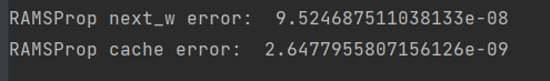
# You should see relative errors around e-7 or less
print('RAMSProp next_w error: ', rel_error(expected_next_w, next_w))
print('RAMSProp cache error: ', rel_error(expected_cache, config['cache']))
In[19]:
# Test Adam implementation
from cs231n.optim import adam
N, D = 4, 5
w = np.linspace(-0.4, 0.6, num=N*D).reshape(N, D)
dw = np.linspace(-0.6, 0.4, num=N*D).reshape(N, D)
m = np.linspace(0.6, 0.9, num=N*D).reshape(N, D)
v = np.linspace(0.7, 0.5, num=N*D).reshape(N, D)
config = {'learning_rate': 1e-2, 'm': m, 'v': v, 't': 5}
next_w, _ = adam(w, dw, config=config)
expected_next_w = np.asarray([
[-0.40094747, -0.34836187, -0.29577703, -0.24319299, -0.19060977],
[-0.1380274, -0.08544591, -0.03286534, 0.01971428, 0.0722929],
[ 0.1248705, 0.17744702, 0.23002243, 0.28259667, 0.33516969],
[ 0.38774145, 0.44031188, 0.49288093, 0.54544852, 0.59801459]])
expected_v = np.asarray([
[ 0.69966, 0.68908382, 0.67851319, 0.66794809, 0.65738853,],
[ 0.64683452, 0.63628604, 0.6257431, 0.61520571, 0.60467385,],
[ 0.59414753, 0.58362676, 0.57311152, 0.56260183, 0.55209767,],
[ 0.54159906, 0.53110598, 0.52061845, 0.51013645, 0.49966, ]])
expected_m = np.asarray([
[ 0.48, 0.49947368, 0.51894737, 0.53842105, 0.55789474],
[ 0.57736842, 0.59684211, 0.61631579, 0.63578947, 0.65526316],
[ 0.67473684, 0.69421053, 0.71368421, 0.73315789, 0.75263158],
[ 0.77210526, 0.79157895, 0.81105263, 0.83052632, 0.85 ]])
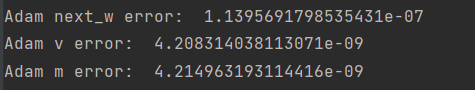
# You should see relative errors around e-7 or less
print('Adam next_w error: ', rel_error(expected_next_w, next_w))
print('Adam v error: ', rel_error(expected_v, config['v']))
print('Adam m error: ', rel_error(expected_m, config['m']))
运行以下命令来训练一对深层网络使用这些新的更新规则:
In[20]:
learning_rates = {'rmsprop': 1e-4, 'adam': 1e-3}
for update_rule in ['adam', 'rmsprop']:
  print('running with ', update_rule)
  model = FullyConnectedNet([100, 100, 100, 100, 100], weight_scale=5e-2)

  solver = Solver(model, small_data,
                  num_epochs=5, batch_size=100,
                  update_rule=update_rule,
                  optim_config={
                    'learning_rate': learning_rates[update_rule]
                  },
                  verbose=True)
  solvers[update_rule] = solver
  solver.train()
  print()

plt.subplot(3, 1, 1)
plt.title('Training loss')
plt.xlabel('Iteration')

plt.subplot(3, 1, 2)
plt.title('Training accuracy')
plt.xlabel('Epoch')

plt.subplot(3, 1, 3)
plt.title('Validation accuracy')
plt.xlabel('Epoch')

for update_rule, solver in list(solvers.items()):
  plt.subplot(3, 1, 1)
  plt.plot(solver.loss_history, 'o', label=update_rule)

  plt.subplot(3, 1, 2)
  plt.plot(solver.train_acc_history, '-o', label=update_rule)

  plt.subplot(3, 1, 3)
  plt.plot(solver.val_acc_history, '-o', label=update_rule)

for i in [1, 2, 3]:
  plt.subplot(3, 1, i)
  plt.legend(loc='upper center', ncol=4)
plt.gcf().set_size_inches(15, 15)
plt.show()

所以Adam比较好一丢丢
内联问题3:
AdaGrad和Adam一样,是一个基于参数的优化方法,它使用以下更新规则:
cache += dw * 2
w+= - learning_rate * dw / (np.sqrt(cache) + eps)
约翰注意到,当他用AdaGrad训练一个网络时,更新变得非常小,他的网络学习速度很慢。用你对AdaGrad更新规则的了解,为什么更新会变得非常小?Adam也会有同样的问题吗?
答:
更新变得非常小,是因为在每次迭代中,我们都把梯度的平方加起来。因此,如果迭代次数很大,那么缓存值将非常大,因为我们正在积累正值(cache += dw2)。因此,当梯度(dw)除以缓存值的平方根(np.sqrt(cache))时,更新将非常小
Adam没有这个问题,因为它使用了平方梯度的指数加权平均(EWA)(这部分基于RMSprop)。也就是说,它以指数的方式累积过去的梯度,把大的权重分配给最近的梯度,把小的权重分配给旧的梯度。除此之外,Adam使用EWA而不是默认的梯度dwm,所以在EWA下的平法梯度的更新很不错*
现在训练我们的终极模型(只是对于我们就学了这么一点来说😅)
在CIFAR-10上训练最好的全连接模型,将最好的模型存储在best_model变量中。我们要求您使用完全连接的网络在验证集上获得至少50%的精度。
如果你仔细的话,应该有可能得到55%以上的正确率
完成BatchNormalization.ipynb 和 Dropout.ipynb
然后我这里是直接放完成后的结果了具体的完成以上两个我会在后谜案发布博客
In[21]:
best_model = None
best_val = -1
################################################################################
# TODO: Train the best FullyConnectedNet that you can on CIFAR-10. You might   #
# find batch/layer normalization and dropout useful. Store your best model in  #
# the best_model variable.                                                     #
################################################################################
# Random Search
for i in range(20):
    ws = 10**np.random.uniform(-2, -1)
    lr = 10**np.random.uniform(-5, -2)
    reg = 10**np.random.uniform(-3, 3)
    model = FullyConnectedNet([100, 100], weight_scale=ws, reg= reg)

    solver = Solver(model, data,
                    num_epochs=10, batch_size=200,
                    update_rule='adam',
                    optim_config={
                      'learning_rate': lr
                    },
                    verbose=False)
    solver.train()
    val_accuracy = solver.best_val_acc
    if best_val < val_accuracy:
        best_val = val_accuracy
        best_model = model
    # Print results
    print('lr %e ws %e reg %e val accuracy: %f' % (
                lr, ws, reg, val_accuracy))
print('best validation accuracy achieved: %f' % best_val)
################################################################################
#                              END OF YOUR CODE                                #
################################################################################

在验证和测试集上运行您的最佳模型。您应该在验证集上达到50%以上的准确性。
In[22]:
y_test_pred = np.argmax(best_model.loss(data['X_test']), axis=1)
y_val_pred = np.argmax(best_model.loss(data['X_val']), axis=1)
print('Validation set accuracy: ', (y_val_pred == data['y_val']).mean())
print('Test set accuracy: ', (y_test_pred == data['y_test']).mean())
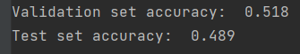
额。。。。这似乎并不是很好
于是我改了一部分参数,如果你的结果也不咋地你也可以多试试,就是耐心奥,反正我边等边刷抖音哈哈哈哈哈

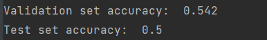
这次就完美卡点


 1444
1444


 被折叠的 条评论
为什么被折叠?
被折叠的 条评论
为什么被折叠?
 到【灌水乐园】发言


