计算机视觉第二章局部图像描述子

鲸~屿

于 2024-08-27 22:36:58 发布

阅读量425

点赞数 8

文章标签：计算机视觉人工智能算法

本文链接：https://blog.csdn.net/qq_53034510/article/details/141508115

版权

2.1 Harris角点检测器

Harris角点检测算法是一个极为简单的角点检测算法。该算法的主要思想是，如果像素周围显示存在多于一个方向的边，我们认为该点为兴趣点，也称为角点。

我们把图像域中点x上的对称半正定矩阵 $M_{I}=M_{I}(x)$ 定义为：

$M_{I}=\bigtriangledown I\bigtriangledown I^{T}=\begin{bmatrix} I_{x}\\ I_{y} \end{bmatrix}\begin{bmatrix} I_{x}& I_{y} \end{bmatrix}=\begin{bmatrix} I_{x}^{2}&I_{x}I_{y} \\ I_{x}I_{y}& I_{y}^{2} \end{bmatrix}$

其中 $\bigtriangledown I$ 为包含导数 $I_{x}$ 和 $I_{y}$ 的图像梯度（我们已经在第1章定义了图像的导数和梯度）。由于该定义， $M_{I}$ 的秩为1，特征值为 $\lambda _{1}=|\bigtriangledown I|^{2}$ 和 $\lambda _{2}=0$ 。选择权重矩阵 $W$ ，可以得到卷积：

$\bar{M_{I}}=W*M_{I}$

该卷积的目的是得到 $M_{I}$ 在周围像素上的局部平均。在不需要实际计算特征值的情况下，为了把重要的情况和其他情况分开，引入了指示函数

$det(\bar{M}_{I})-\kappa trace(\bar{M}_{I})^{2}$

为了去除加权常数 $\kappa$ ，通常改为商数作为指示器，即

$\frac{det(\bar{M}_{I})}{trace(\bar{M}_{I})^{2}}$

下面编写Harris角点检测程序

import numpy as np
from scipy.ndimage import gaussian_filter
from PIL import Image
import matplotlib.pyplot as plt


def compute_harris_response(im, sigma=3):
    """在一幅灰度图像中，对每一个像素计算Harris角点检测器响应函数"""

    # 计算导数
    imx = np.zeros(im.shape)
    gaussian_filter(im, (sigma, sigma), (0, 1), imx)

    imy = np.zeros(im.shape)
    gaussian_filter(im, (sigma, sigma), (1, 0), imy)

    # 计算 Harris 矩阵的分量
    Wxx = gaussian_filter(imx * imx, sigma)
    Wxy = gaussian_filter(imx * imy, sigma)
    Wyy = gaussian_filter(imy * imy, sigma)

    # 计算特征值和迹
    Wdet = Wxx * Wyy - Wxy * Wxy
    Wtr = Wxx + Wyy

    return Wdet / Wtr


def get_harris_points(harrisim, min_dist=10, threshold=0.1):
    """从一幅Harris响应图像中返回角点，min_dist为分割角点和图像边界的最少像素数目"""

    # 寻找高于阈值的候选角点
    corner_threshold = harrisim.max() * threshold
    harrisim_t = (harrisim > corner_threshold) * 1

    # 得到候选点的坐标
    coords = np.array(harrisim_t.nonzero()).T

    # 以及它们的 Harris 响应值
    candidate_values = [harrisim[c[0], c[1]] for c in coords]

    # 对候选点按照 Harris 响应值进行排序
    index = np.argsort(candidate_values)

    # 将可行点的位置保存到数组中
    allowed_locations = np.zeros(harrisim.shape)
    allowed_locations[min_dist:-min_dist, min_dist:-min_dist] = 1

    # 按照 min_distance 原则，选择最佳 Harris 点
    filtered_coords = []
    for i in index:
        if allowed_locations[coords[i][0], coords[i][1]] == 1:
            filtered_coords.append(coords[i])
            allowed_locations[coords[i][0] - min_dist:coords[i][0] + min_dist,
            coords[i][1] - min_dist:coords[i][1] + min_dist] = 0
    return filtered_coords


if __name__ == "__main__":
    # 读取图像
    im = np.array(Image.open('eg.jpg').convert('L'))

    # 计算 Harris 响应
    harrisim = compute_harris_response(im)
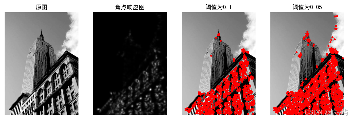
    filtered_coords1 = get_harris_points(harrisim, min_dist=6, threshold=0.1)
    filtered_coords2 = get_harris_points(harrisim, min_dist=6, threshold=0.05)

    # 显示结果并保存图像
    plt.rcParams['font.sans-serif'] = ['SimHei']
    plt.subplot(151), plt.imshow(im, cmap='gray'), plt.title('原图'), plt.axis('off')
    plt.subplot(152), plt.imshow(harrisim, cmap='gray'), plt.title('角点响应图'), plt.axis('off')
    plt.subplot(153), plt.imshow(im, cmap='gray'), plt.plot([p[1] for p in filtered_coords1],
                                                            [p[0] for p in filtered_coords1], 'r.'),
    plt.title('阈值为0.1'), plt.axis('off')
    plt.subplot(154), plt.imshow(im, cmap='gray'), plt.plot([p[1] for p in filtered_coords2],
                                                            [p[0] for p in filtered_coords2], 'r.'),
    plt.title('阈值为0.05'), plt.axis('off')

    # 保存图像为文件
    plt.savefig('harris.jpg', dpi=300, bbox_inches='tight')

    # 显示图像
    plt.show()

其运行结果如下图所示：

2.2 SIFT（尺度不变特征变换）

SIFT（尺度不变特征变换，Scale-Invariant Feature Transform）是一种用于图像特征提取和描述的计算机视觉算法。它可以有效地检测和描述图像中的局部特征，具有对图像缩放、旋转和光照变化的较强不变性。

2.2.1 兴趣点

SIFT 特征使用高斯差分函数来定位兴趣点：

$D(x,\sigma )=[G_{\kappa \sigma }(x)-G_{\sigma }(x)]*I(x)=[G_{\kappa \sigma }-G_{\sigma }]*I=I_{\kappa \sigma}-I_{\sigma }$

其中， $G_{\sigma }$ 是二维高斯核， $I_{\sigma }$ 是使用 $G_{\sigma }$ 模糊的灰度图像， $\kappa$ 是决定相差尺度的常数。兴趣点是在图像位置和尺度变化下 $D(x,\sigma )$ 的最大值和最小值点。

2.2.2 描述子

SIFT描述子在每个像素点附近选取子区域网格，在每个子区域内计算图像梯度方向直方图，每个子区域的直方图拼接起来组成描述子向量。

2.2.3 检测兴趣点

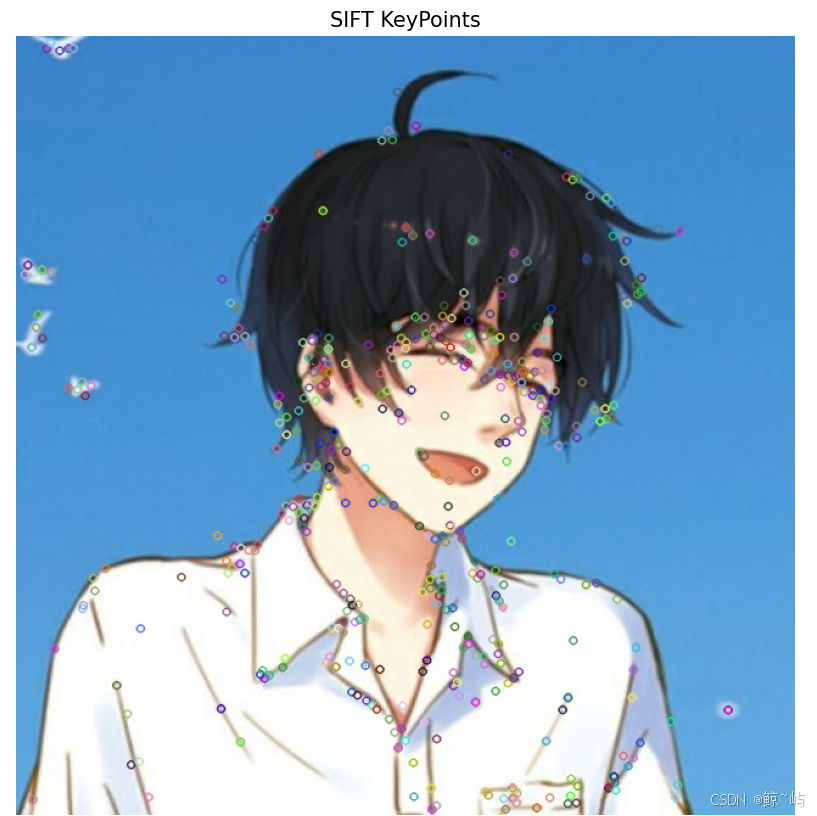
我们使用书上的示例代码运行不出来，故使用opencv库来检测兴趣点，运行代码如下所示：

import cv2
import numpy as np
import matplotlib.pyplot as plt

def detect_and_plot_features(image_path):
    # 读取图像并转换为灰度
    image = cv2.imread(image_path)
    gray_image = cv2.cvtColor(image, cv2.COLOR_BGR2GRAY)

    # 创建 SIFT 检测器
    sift = cv2.SIFT_create()

    # 检测 SIFT 特征点
    keypoints, descriptors = sift.detectAndCompute(gray_image, None)

    # 绘制特征点
    image_with_keypoints = cv2.drawKeypoints(image, keypoints, None)

    # 显示图像
    plt.figure(figsize=(10, 10))
    plt.imshow(cv2.cvtColor(image_with_keypoints, cv2.COLOR_BGR2RGB))
    plt.axis('off')
    plt.title('SIFT KeyPoints')
    plt.show()

# 调用函数
detect_and_plot_features('touxiang.jpg')  # 替换为您自己的图像路径

绘制出的SIFT特征位置图像如下所示：

2.2.4 匹配描述子

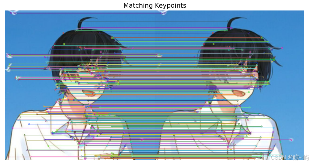
在计算机视觉中，描述子匹配是特征匹样本分析中的一个重要步骤，特别是在图像匹配和物体识别任务中。描述子匹配的核心思想是找到两个图像之间相似的特征点，并用相应的描述子进行匹配。以下是使用 OpenCV 进行描述子匹配的示例代码，采用 SIFT 特征。

import cv2
import numpy as np
import matplotlib.pyplot as plt


def match_descriptors(image1_path, image2_path):
    # 读取图像并转换为灰度
    img1 = cv2.imread(image1_path)
    img2 = cv2.imread(image2_path)

    gray1 = cv2.cvtColor(img1, cv2.COLOR_BGR2GRAY)
    gray2 = cv2.cvtColor(img2, cv2.COLOR_BGR2GRAY)

    # 创建 SIFT 检测器
    sift = cv2.SIFT_create()

    # 检测特征点及计算描述子
    keypoints1, descriptors1 = sift.detectAndCompute(gray1, None)
    keypoints2, descriptors2 = sift.detectAndCompute(gray2, None)

    # 使用 BFMatcher 进行匹配
    bf = cv2.BFMatcher(cv2.NORM_L2)  # 使用 L2 距离
    matches = bf.knnMatch(descriptors1, descriptors2, k=2)  # 找到每个描述子的 2 个最佳匹配

    # 筛选出良好的匹配（比率测试）
    good_matches = []
    for m, n in matches:
        if m.distance < 0.75 * n.distance:  # Lowe's ratio test
            good_matches.append(m)

            # 绘制匹配结果
    match_image = cv2.drawMatches(img1, keypoints1, img2, keypoints2, good_matches, None,
                                  flags=cv2.DrawMatchesFlags_NOT_DRAW_SINGLE_POINTS)

    plt.figure(figsize=(10, 10))
    plt.imshow(cv2.cvtColor(match_image, cv2.COLOR_BGR2RGB))
    plt.axis('off')
    plt.title('Matching Keypoints')
    plt.show()


# 调用函数，替换图像路径
match_descriptors('touxiang.jpg', 'touxiang.jpg')  # 替换为您自己的图像路径

匹配结果如下图

2.3 匹配地理标记图像

我们使用局部描述子来匹配带有地理标记的图像。

2.3.1 从百度地图下载地理标记图像

从百度地图下载地理标记图像的过程涉及 API 的使用，但百度地图的 API 并不直接支持下载图像。通常情况下，我们可以从地图 API 获取地理标记、位置信息及其相关图像的链接，然后手动下载或使用 Python 下载图像。

1.获取百度地图 API 密钥

在使用百度地图 API 之前，您需要先注册一个百度开发者账户并申请一个 API 密钥。可以访问https://lbsyun.baidu.com来申请。

2.使用 Python 获取相关数据

以下是一个基本的示例，展示如何使用 Python 和百度地图 API 查找某个地点的位置信息，并下载该地点的静态地图图像。

import requests  
import os  

# 百度地图 API 配置  
AK = 'YOUR_BAIDU_MAP_API_KEY'  # 替换为您的 API 密钥  
location = '39.915,116.404'  # 替换为目标地理位置的经纬度，例如北京的经纬度  

# 构建百度地图静态地图 API 请求 URL  
map_url = f'http://api.map.baidu.com/staticimage/v2?ak={AK}&center={location}&width=600&height=400&markers={location}&markerStyles=l,red&zoom=12'  

# 发起请求并下载图像  
response = requests.get(map_url)  

# 创建用于保存图像的目录  
os.makedirs('baidu_maps', exist_ok=True)  

# 指定保存的文件名  
image_path = os.path.join('baidu_maps', 'map_image.jpg')  

# 保存图像  
with open(image_path, 'wb') as file:  
    file.write(response.content)  

print(f"地图图像已下载到: {image_path}")

2.3.2 使用局部描述子匹配

我们刚才已经下载了这些图像，下面需要对这些图像提取局部描述子。在这种情况下，我们将使用前面部分讲述的SIFT特征描述子。

import sift
nbr_images = len(imlist)
matchscores = zeros((nbr_images,nbr_images))
for i in range(nbr_images):
    for j in range(i,nbr_images): # 仅仅计算上三角
        print('comparing', imlist[i], imlist[j])
        l1, d1 = sift.read_features_from_file(featlist[i])
        l2, d2 = sift.read_features_from_file(featlist[j])
        matches = sift.match_twosided(d1, d2)
        nbr_matches = sum(matches > 0)
        print('number of matches = ', nbr_matches)
        matchscores[i, j] = nbr_matches
# 复制值
for i in range(nbr_images):
    for j in range(i + 1, nbr_images):  # 不需要复制对角线
        matchscores[j, i] = matchscores[i, j]

2.3.3 可视化连接图像

为了可视化连接通过局部特征匹配找到的图像，您可以使用 OpenCV 将匹配的特征绘制在一起。下述步骤将展示如何使用 Python 和 OpenCV 可视化连接匹配的图像。

import cv2  
import numpy as np  

# 加载图像  
img1 = cv2.imread('baidu_maps/map_image.jpg')  # 百度地图图像  
img2 = cv2.imread('your_other_image.jpg')  # 要匹配的另一张图像  

# 转换为灰度图  
gray1 = cv2.cvtColor(img1, cv2.COLOR_BGR2GRAY)  
gray2 = cv2.cvtColor(img2, cv2.COLOR_BGR2GRAY)  

# 创建 ORB 检测器  
orb = cv2.ORB_create()  

# 找到关键点和描述子  
keypoints1, descriptors1 = orb.detectAndCompute(gray1, None)  
keypoints2, descriptors2 = orb.detectAndCompute(gray2, None)  

# 创建 BFMatcher 对象  
bf = cv2.BFMatcher(cv2.NORM_HAMMING, crossCheck=True)  

# 匹配描述子  
matches = bf.match(descriptors1, descriptors2)  

# 排序匹配结果  
matches = sorted(matches, key=lambda x: x.distance)  

# 获取关键点的位置  
points1 = np.zeros((len(matches), 2), dtype=np.float32)  
points2 = np.zeros((len(matches), 2), dtype=np.float32)  

for i, match in enumerate(matches):  
    points1[i, :] = keypoints1[match.queryIdx].pt  # 图像1的关键点  
    points2[i, :] = keypoints2[match.trainIdx].pt  # 图像2的关键点  

# 连接图像  
# 创建一个新图像，宽度为两幅图像的宽度之和  
height = max(img1.shape[0], img2.shape[0])  
new_width = img1.shape[1] + img2.shape[1]  
result = np.zeros((height, new_width, 3), dtype=np.uint8)  
result[:img1.shape[0], :img1.shape[1]] = img1  
result[:img2.shape[0], img1.shape[1]:] = img2  

# 绘制匹配结果  
for i in range(len(matches)):  
    pt1 = (int(points1[i, 0]), int(points1[i, 1]))  
    pt2 = (int(points2[i, 0]) + img1.shape[1], int(points2[i, 1]))  
    cv2.line(result, pt1, pt2, (0, 255, 0), 1)  # 绘制线条，颜色为绿色  

# 显示结果  
cv2.imshow("Matched Image", result)  
cv2.waitKey(0)  
cv2.destroyAllWindows()

鲸~屿

关注

8
点赞
踩
15

收藏

觉得还不错? 一键收藏
0
评论
计算机视觉第二章局部图像描述子

描述子匹配的核心思想是找到两个图像之间相似的特征点，并用相应的描述子进行匹配。它可以有效地检测和描述图像中的局部特征，具有对图像缩放、旋转和光照变化的较强不变性。从百度地图下载地理标记图像的过程涉及 API 的使用，但百度地图的 API 并不直接支持下载图像。SIFT描述子在每个像素点附近选取子区域网格，在每个子区域内计算图像梯度方向直方图，每个子区域的直方图拼接起来组成描述子向量。以下是一个基本的示例，展示如何使用 Python 和百度地图 API 查找某个地点的位置信息，并下载该地点的静态地图图像。
复制链接

扫一扫