【金融量化分析】#Financial Computation（利率、债券、期权相关数理知识与代码实现)

本篇文章涉及到的金融衍生品的计算，主要分为一下几个大类。👇flow chart

子：Bond债券相关计算

在此之前先回顾一下金融衍生品相关利率的知识。点这里上车🚗

一：rates的计算

1：Effective return

two ways to calculate the average of return
1）arithmetic average
2) geometric average

Head:
Tom and Amy both bought a 20-year pension with different return schemes. Tom’s pension has first year interest rate of 3% and will increase by 0.5% every year whilst Amy’s pension has a continuous interest rate of 7%. Both pension pays the interest annually. Compare the benefits of the two pensions by computing their effective rates of return.

%% Solution:
InterestR_Tom=[3:0.5:12.5]/100;
EffectiveR_Tom=(prod(1+[3:0.5:12.5]/100))^(1/20)-1;% 用平均来算
EffectiveR_Tom=prod(

EffectiveR_AMY=exp(0.07)-1;

if EffectiveR_Tom>EffectiveR_AMY
    disp('The pension of Tom has higher effective rate')
elseif EffectiveR_Tom<EffectiveR_AMY
    disp('The pension of Amy has higher effective rate')
else
    disp('The effective rates are equal')
end
   

二：Bondprice; Duration and convexity

编程思路：
首先wirte a user_defined matlab-code and call it 来计算Price,duration,convexity
then根据portifolio的性质进行编程

function [Price,duration,convexity] = DurationConvexity(Face,Coupon,Maturity,yield)
% BondPrice, Duration and Convexity
    Time=0.5:0.5:Maturity; % time for payments
    C = 0.5*Coupon*Face; % one coupon payment
    Price = sum(C*exp(-yield*Time)) + Face*exp(-yield*Maturity);
    duration= sum( (C* Time.* exp(-yield*Time) )/ Price )+Face*Maturity*exp(-yield*Maturity)/Price;
    convexity = sum( (C.* (Time.^2).* exp(-yield*Time) )./ Price )+Face*(Maturity^2)*exp(-yield*Maturity)/Price;
end

Head:
Suppose you have two bonds in your portfolio, i.e. bond A and bond B, where both bonds have semi-annual coupon payments with annual coupon rates 4% and 5%, the maturities are 2 and 3 years, respectively. Both bonds have face value of 100 and the yields of these two bonds are given as 5% and 6.5%.
1、Calculate the value of your bond portfolio.
2、Calculate the duration of your bond portfolio.
3、Calculate the convexity of your bond portfolio.
4、Using the first order approximation and second order approximations calculate the relative change in the value of your bond portfolio if the yields go up with 25 basis points (25 basis points means 0.25%).

%% (a)

[price_A,duration_A,convexity_A] = DurationConvexity(100,0.04,2,0.05);
[price_B,duration_B,convexity_B] = DurationConvexity(100,0.05,3,0.065);

price_Portfolio=price_A+price_B

%% (b)

w_A=price_A/price_Portfolio;
w_B=price_B/price_Portfolio;

duration_Portfolio=w_A*duration_A+w_B*duration_B
%% calculate the weight of each asset multiply duration respectively

%% (c)

convexity_Portfolio=w_A*convexity_A+w_B*convexity_B

%% (d)

% first order approximation  % 1st taylor expansion

PriceChange1=-0.0025*duration_Portfolio;

% second order approximation

PriceChange2=-0.0025*duration_Portfolio+0.5*(0.0025)^2*convexity_Portfolio;

#https://www.docin.com/p-35161143.html 一个问题

三：bootstrap 法 and related rates的计算

1：bootstrapping method

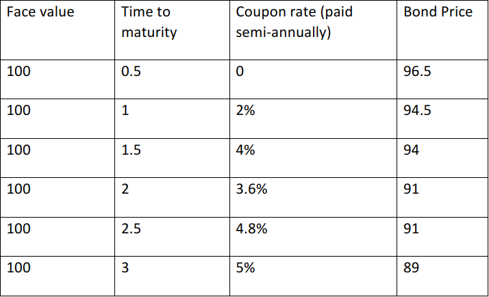
(a) Use Table 1 to calculate the zero rates using the bootstrapping method. Note that coupon rates are annual rates with semi-annual payments. For example, 2% per annum coupon rate means 1 dollar payment every six months for the face value of 100 dollars.

2：implied forward rates

(b) Calculate the implied forward rates using the zero rates obtained from 1 to 2 years and from 2 to 3 years time periods.

3：par yields

(c ) Calculate the par yields for the 1, 2, and 3 year maturities using the zero rates obtained.

4：duration and convexity

(d) Calculate the duration and convexity of the 3-year bond using the definition of duration and convexity.

5： approximation

(e) Suppose that the yields increase by 25 basis points (i.e. increase by 0.25%), then use the duration to approximate the change in the relative value of the 3-year bond. Second, use the duration and convexity to approximate the change in the relative value of the 3- year bond.

6：price change

(f) Now using your first order and second order approximations obtained in the previous part compare the approximations with the exact relative change in the value of the bond.

%% Solution A:
F=100
M=[0.5:0.5:3]
Cr=[0 2 4 3.6 4.8 5]/100
Coupon=Cr.*F/2;
BP=[96.5 94.5 94 91 91 89];
ZeroRate=[]
for i=1:length(Cr);
    PaymentTime2=M(1:i); %t are the points of cash flows
    ZeroRate(i)=(log(F+Coupon(i))-log(BP(i)-sum(Coupon(i)*exp(-ZeroRate(1:i-1).*PaymentTime2(1:end-1)))))/M(i);
end
Time_grid=[0.05:0.05:3];
R_spline=interp1(M,ZeroRate,Time_grid,'spline');
plot(M,ZeroRate,'o',Time_grid,R_spline,'r'),xlabel('Time'),ylabel('Zero rates'),title('Spline interpolation')

%% Solution B:

ForwardRate1=2*ZeroRate(4)-1*ZeroRate(2)

ForwardRate2=3*ZeroRate(6)-2*ZeroRate(4)

%% Solution C:

Discount1=exp(-1.*ZeroRate(2));
Discount2=exp(-2*ZeroRate(4));
Discount3=exp(-3*ZeroRate(6));

ParY1=(1-Discount1)/Discount1
ParY2=(1-Discount2)/sum([Discount1,Discount2])
ParY3=(1