Ceres简介及示例（2）helloworld 自动梯度求导、数值求导、解析法求导

1、Ceres目标

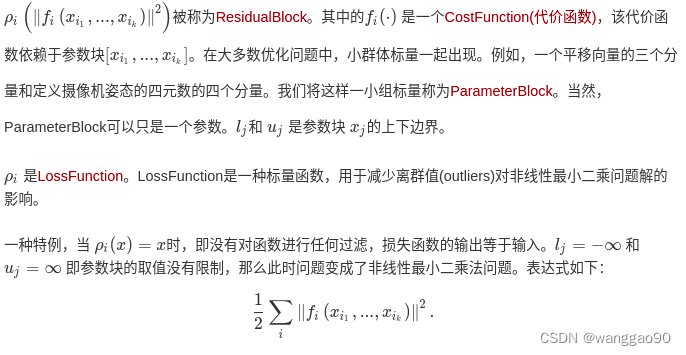
Ceres 可以解决以下形式的边界约束鲁棒化非线性最小二乘问题，

$$\begin{array}{rl}\underset{\mathbf{x}}{\min }& \frac{1}{2}\sum _i{\rho }_i\left({\Vert f_i\left(x_{i_1},...,x_{i_k}\right)\Vert }^2\right)\\ \text{s.t.}& l_j\le x_j\le u_j\end{array}$$
目标 $mi{n}_{x}f(x)$ 是通过优化算法，计算得到一个$x$使$f(x)$取得最小值。这一表达式在工程和科学领域有非常广泛的应用。比如统计学中的曲线拟合，或者在计算机视觉中依据图像进行三维模型的构建等等。

深度学习中，我们将残差Residual称为优化目标函数，代价函数为误差函数。

1.1、标量

单个数值，基本很简单，可以认为是一个只有一个元素的向量。

1.2、向量

常规曲线函数拟合的结果， 也可以认为是多个标量组成的。

1.3、矩阵

可以理解为优化目标是由多个向量组合的，例如相机姿态、相机内参等。

2、helloworld - Automatic Differentiation（自动梯度求导）

考虑一个简单问题， 待求解直线 y(x) = x， 目标直线 y = 10，问x取值多少时，y(x)和y差异最小？

显而易见，x=10就是我们需要优化的结果。简单地选择损失函数取 $\rho =x$，此时的代价函数，
$$\begin{gathered} 目标函数{\rho }_x=mi{n}_x\frac{1}{2}(10-x{)}^2 \\ 残差f(x)=y-y(x)=10-x \end{gathered}$$

（1）首先，编写一个函子来评估这个函数 $f(x)=10-x$

// 构建代价函数，重载()符号
struct CostFunctor {
   template <typename T>
   bool operator()(const T* const x, T* residual) const {
     residual[0] = 10.0 - x[0];
     return true;
   }
};

operator()是一个模板化方法，它假定其所有输入和输出都是某种类型T。这里使用模板允许Ceres调用CostFunctor::operator()，当只需要残差值时使用T=double，当需要雅可比矩阵时使用特殊类型T=Jet。

一旦我们有了计算残差函数的方法，现在是时候用它来构造一个非线性最小二乘问题并让Ceres来解决它了。主体函数代码

#include "ceres/ceres.h"
#include "glog/logging.h"

using ceres::AutoDiffCostFunction;
using ceres::CostFunction;
using ceres::Problem;
using ceres::Solver;
using ceres::Solve;

// A templated cost functor that implements the residual r = 10 -
// x. The method operator() is templated so that we can then use an
// automatic differentiation wrapper around it to generate its
// derivatives.
// 第一部分：构建代价函数，重载()符号，仿函数的小技巧
struct CostFunctor {
  template <typename T> bool operator()(const T* const x, T* residual) const {
    residual[0] = 10.0 - x[0];
    return true;
  }
};

int main(int argc, char** argv) {
  google::InitGoogleLogging(argv[0]);

  // 设置寻优参数x的初始值，为0.5
  double initial_x = 5.0;
  double x = initial_x;

  // 第二部分：构建寻优问题
  Problem problem;

  // 使用自动求导，将之前的代价函数结构体传入，第一个1是输出维度，即残差的维度，第二个1是输入维度，即待寻优参数x的维度。
  CostFunction* cost_function =
      new AutoDiffCostFunction<CostFunctor, 1, 1>(new CostFunctor); // 自动求导梯度
  // 向问题中添加残差项，本问题比较简单，添加一个就行。
  problem.AddResidualBlock(cost_function, nullptr, &x);

  // 第三部分： 配置并运行求解器
  Solver::Options options;
  options.minimizer_progress_to_stdout = true;
  
  Solver::Summary summary;// 优化信息
  Solve(options, &problem, &summary);// 求解

  std::cout << summary.BriefReport() << "\n"; // 输出优化的简要信息
  std::cout << "x : " << initial_x
            << " -> " << x << "\n";
  return 0;
}

运行结果

iter      cost      cost_change  |gradient|   |step|    tr_ratio  tr_radius  ls_iter  iter_time  total_time
   0  4.512500e+01    0.00e+00    9.50e+00   0.00e+00   0.00e+00  1.00e+04        0    2.86e-04    8.84e-04
   1  4.511598e-07    4.51e+01    9.50e-04   9.50e+00   1.00e+00  3.00e+04        1    3.63e-04    2.03e-03
   2  5.012552e-16    4.51e-07    3.17e-08   9.50e-04   1.00e+00  9.00e+04        1    1.80e-04    2.33e-03
Ceres Solver Report: Iterations: 3, Initial cost: 4.512500e+01, Final cost: 5.012552e-16, Termination: CONVERGENCE
x : 0.5 -> 10

初始值为0.5，最终通过3次循环之后到达最优解10。其实本例是一个线性问题，因为
f(x)=10−x是一个线性函数，但是Ceres仍然可以应用。对于Ceres解非线性应用的流程和具体配置将在后续的教程中给出。

1.构建代价函数
使用了仿函数，即在CostFunctor结构体内，对()操作符进行了重载，这样使该结构体的一个实例就能具有类似一个函数的性质，在代码编写过程中就能当做一个函数一样来使用。

注意，这里的残差是当前输入x值与目标y=10的插值。

2.配置问题并求解问题
Solver::Options定义了非常多的默认参数，用来配置求解器solver如何运行优化算法。关注，options.linear_solver_type参数，代码中为

#if defined(CERES_NO_SUITESPARSE) && defined(CERES_NO_CXSPARSE) && !defined(CERES_ENABLE_LGPL_CODE)  // NOLINT
      linear_solver_type = DENSE_QR;
#else
      linear_solver_type = SPARSE_NORMAL_CHOLESKY;
#endif

当不使用SuiteSparse, CXSparse等库是，默认使用SPARSE_NORMAL_CHOLESKY求解，如果修改为 DENSE_QR将报错

solver.cc:531 Terminating: Can't use SPARSE_NORMAL_CHOLESKY with SUITESPARSE because SuiteSparse was not enabled when Ceres was built.

线性求解器的类型，用于计算Levenberg-Marquardt算法每次迭代中线性最小二乘问题的解。

• DENSE_QR:
  对于较小的问题(几百个参数和几千个残差)，相对稠密的Jacobians，DENSE_QR 是一个选择。
• DENSE_NORMAL_CHOLESKY & SPARSE_NORMAL_CHOLESKY:
  大型非线性最小二乘问题通常是稀疏的。在这种情况下，使用稠密的QR分解是低效的。

2、helloworld - Numeric Derivatives(数值法求导)

某些情况下，不能用模板形式定义仿函数，例如，当残差的求值涉及调用您无法控制的库函数时。在这种情况下，可以使用数值微分法。用户定义一个仿函数(functor)来计算残差值，并且构建一个数值微分代价函数(NumericDiffCostFunction)。

比如对于 f(x)=10−x 对应函数体如下：

/*
对比Helloworld中的Functor的定义发现，这次没用模板类。
*/
struct NumericDiffCostFunctor {
  bool operator()(const double* const x, double* residual) const {
    residual[0] = 10.0 - x[0];
    return true;
  }
};

再添加到Problem中

CostFunction* cost_function =
  new NumericDiffCostFunction<NumericDiffCostFunctor, ceres::CENTRAL, 1, 1>(
      new NumericDiffCostFunctor);
problem.AddResidualBlock(cost_function, nullptr, &x);

对比在Hello World中使用automatic differentiation算法，

CostFunction* cost_function =
    new AutoDiffCostFunction<CostFunctor, 1, 1>(new CostFunctor);
problem.AddResidualBlock(cost_function, nullptr, &x);

发现两种算法在构建Problem时候基本差不多。但是在用Nummeric算法时需要额外给定一个参数ceres::CENTRAL 。这个参数告诉计算机如何计算导数。

一般来说，Ceres官方更加推荐自动微分算法，因为C++模板类使自动算法有更高的效率。数值微分算法通常来说计算更复杂，收敛更缓慢。

完整代码

#include "ceres/ceres.h"
#include "glog/logging.h"

using ceres::NumericDiffCostFunction;
using ceres::CENTRAL;
using ceres::CostFunction;
using ceres::Problem;
using ceres::Solver;
using ceres::Solve;

// A cost functor that implements the residual r = 10 - x.
struct CostFunctor {
  bool operator()(const double* const x, double* residual) const {
    residual[0] = 10.0 - x[0];
    return true;
  }
};

int main(int argc, char** argv) {
  google::InitGoogleLogging(argv[0]);

  // The variable to solve for with its initial value. It will be
  // mutated in place by the solver.
  double x = 0.5;
  const double initial_x = x;

  // Build the problem.
  Problem problem;

  // Set up the only cost function (also known as residual). This uses
  // numeric differentiation to obtain the derivative (jacobian).
  CostFunction* cost_function =
      new NumericDiffCostFunction<CostFunctor, CENTRAL, 1, 1> (new CostFunctor);
  problem.AddResidualBlock(cost_function, NULL, &x);

  // Run the solver!
  Solver::Options options;
  options.minimizer_progress_to_stdout = true;
  options.linear_solver_type = ceres::DENSE_QR;
  Solver::Summary summary;
  Solve(options, &problem, &summary);

  std::cout << summary.BriefReport() << "\n";
  std::cout << "initial x : " << initial_x << ", "
            << "result x : " << x << "\n";
  return 0;
}

3、helloworld - Analytic Derivatives(解析法求导)

有些时候，应用自动求解算法时不可能的。比如在某些情况下，计算导数的时候，使用闭合解（closed form，也被称为解析解）会比使用自动微分算法中的链式法则（chain rule）更有效率。

在这种情况下，需要编写残差和雅可比行列式的计算代码了。为此，定义一个CostFunction的子类，或者在编译时知道了参数的大小和残差，则可以定义SizedCostFunction的子类。

例如，为了实现f(x) = 10 - x，有一个简单的例子

class QuadraticCostFunction : public ceres::SizedCostFunction<1, 1> {
 public:
  virtual ~QuadraticCostFunction() {}
  virtual bool Evaluate(double const* const* parameters,
                        double* residuals,
                        double** jacobians) const {
    const double x = parameters[0][0];
    residuals[0] = 10 - x;

    // 计算雅克比矩阵，目前只有一个值
    if (jacobians != nullptr && jacobians[0] != nullptr) {
      jacobians[0][0] = -1;    // dr/dx
    }
    return true;
  }
};

parameters：输入数组参数
residuals/jacobians：输出数组参数
Evaluate()用于检查jacobians是否为非空值。如果不为空，那么就把残差方程的导数值赋值给它。在这种情况下，由于残差函数是线性的，雅可比矩阵是常数。

从上面的代码片段可以看出，实现CostFunction对象有点繁琐。我们建议，除非有特殊的原因自己管理雅可比矩阵计算，否则您可以使用AutoDiffCostFunction或NumericDiffCostFunction来构造残差块。

注意区别：示例中单个元素传递只用指针，仿函数通过一维下标访问；当使用SizedCostFunction时，输入参数被转换成二维数组指针。

完整代码

#include <vector>
#include "ceres/ceres.h"
#include "glog/logging.h"

using ceres::CostFunction;
using ceres::SizedCostFunction;
using ceres::Problem;
using ceres::Solver;
using ceres::Solve;

// A CostFunction implementing analytically derivatives for the
// function f(x) = 10 - x.
class QuadraticCostFunction
  : public SizedCostFunction<1 /* number of residuals */,
                             1 /* size of first parameter */> {
 public:
  virtual ~QuadraticCostFunction() {}

  virtual bool Evaluate(double const* const* parameters,
                        double* residuals,
                        double** jacobians) const {
    double x = parameters[0][0];

    // f(x) = 10 - x.
    residuals[0] = 10 - x;

    // f'(x) = -1. Since there's only 1 parameter and that parameter
    // has 1 dimension, there is only 1 element to fill in the
    // jacobians.
    //
    // Since the Evaluate function can be called with the jacobians
    // pointer equal to NULL, the Evaluate function must check to see
    // if jacobians need to be computed.
    //
    // For this simple problem it is overkill to check if jacobians[0]
    // is NULL, but in general when writing more complex
    // CostFunctions, it is possible that Ceres may only demand the
    // derivatives w.r.t. a subset of the parameter blocks.
    if (jacobians != NULL && jacobians[0] != NULL) {
      jacobians[0][0] = -1;
    }

    return true;
  }
};

int main(int argc, char** argv) {
  google::InitGoogleLogging(argv[0]);

  // The variable to solve for with its initial value. It will be
  // mutated in place by the solver.
  double x = 0.5;
  const double initial_x = x;

  // Build the problem.
  Problem problem;

  // Set up the only cost function (also known as residual).
  CostFunction* cost_function = new QuadraticCostFunction;
  problem.AddResidualBlock(cost_function, NULL, &x);

  // Run the solver!
  Solver::Options options;
  options.minimizer_progress_to_stdout = true;
  options.linear_solver_type = ceres::DENSE_QR;
  Solver::Summary summary;
  Solve(options, &problem, &summary);

  std::cout << summary.BriefReport() << "\n";
  std::cout << "initial x : " << initial_x << ", "
            << "result x : " << x << "\n";

  return 0;
}